
A black theme for ggplot graphics inspired by a blog post of Jon Lefcheck (https://jonlefcheck.net/2013/03/11/black-theme-for-ggplot2-2/).
Details
When using theme_black in plots powered by the
bayesplot package such as pp_check or stanplot,
I recommend using the "viridisC" color scheme (see examples).
Examples
# \dontrun{
# change default ggplot theme
ggplot2::theme_set(theme_black())
#> Warning: 'theme_black' is deprecated. Please use the 'ggdark' package for dark ggplot themes.
#> Warning: The `size` argument of `element_line()` is deprecated as of ggplot2 3.4.0.
#> ℹ Please use the `linewidth` argument instead.
#> ℹ The deprecated feature was likely used in the brms package.
#> Please report the issue at <https://github.com/paul-buerkner/brms/issues>.
# change default bayesplot color scheme
bayesplot::color_scheme_set("viridisC")
# fit a simple model
fit <- brm(count ~ zAge + zBase * Trt + (1|patient),
data = epilepsy, family = poisson(), chains = 2)
#> Compiling Stan program...
#> Start sampling
#>
#> SAMPLING FOR MODEL 'anon_model' NOW (CHAIN 1).
#> Chain 1:
#> Chain 1: Gradient evaluation took 3.2e-05 seconds
#> Chain 1: 1000 transitions using 10 leapfrog steps per transition would take 0.32 seconds.
#> Chain 1: Adjust your expectations accordingly!
#> Chain 1:
#> Chain 1:
#> Chain 1: Iteration: 1 / 2000 [ 0%] (Warmup)
#> Chain 1: Iteration: 200 / 2000 [ 10%] (Warmup)
#> Chain 1: Iteration: 400 / 2000 [ 20%] (Warmup)
#> Chain 1: Iteration: 600 / 2000 [ 30%] (Warmup)
#> Chain 1: Iteration: 800 / 2000 [ 40%] (Warmup)
#> Chain 1: Iteration: 1000 / 2000 [ 50%] (Warmup)
#> Chain 1: Iteration: 1001 / 2000 [ 50%] (Sampling)
#> Chain 1: Iteration: 1200 / 2000 [ 60%] (Sampling)
#> Chain 1: Iteration: 1400 / 2000 [ 70%] (Sampling)
#> Chain 1: Iteration: 1600 / 2000 [ 80%] (Sampling)
#> Chain 1: Iteration: 1800 / 2000 [ 90%] (Sampling)
#> Chain 1: Iteration: 2000 / 2000 [100%] (Sampling)
#> Chain 1:
#> Chain 1: Elapsed Time: 2.054 seconds (Warm-up)
#> Chain 1: 1.529 seconds (Sampling)
#> Chain 1: 3.583 seconds (Total)
#> Chain 1:
#>
#> SAMPLING FOR MODEL 'anon_model' NOW (CHAIN 2).
#> Chain 2:
#> Chain 2: Gradient evaluation took 2.5e-05 seconds
#> Chain 2: 1000 transitions using 10 leapfrog steps per transition would take 0.25 seconds.
#> Chain 2: Adjust your expectations accordingly!
#> Chain 2:
#> Chain 2:
#> Chain 2: Iteration: 1 / 2000 [ 0%] (Warmup)
#> Chain 2: Iteration: 200 / 2000 [ 10%] (Warmup)
#> Chain 2: Iteration: 400 / 2000 [ 20%] (Warmup)
#> Chain 2: Iteration: 600 / 2000 [ 30%] (Warmup)
#> Chain 2: Iteration: 800 / 2000 [ 40%] (Warmup)
#> Chain 2: Iteration: 1000 / 2000 [ 50%] (Warmup)
#> Chain 2: Iteration: 1001 / 2000 [ 50%] (Sampling)
#> Chain 2: Iteration: 1200 / 2000 [ 60%] (Sampling)
#> Chain 2: Iteration: 1400 / 2000 [ 70%] (Sampling)
#> Chain 2: Iteration: 1600 / 2000 [ 80%] (Sampling)
#> Chain 2: Iteration: 1800 / 2000 [ 90%] (Sampling)
#> Chain 2: Iteration: 2000 / 2000 [100%] (Sampling)
#> Chain 2:
#> Chain 2: Elapsed Time: 2.255 seconds (Warm-up)
#> Chain 2: 1.542 seconds (Sampling)
#> Chain 2: 3.797 seconds (Total)
#> Chain 2:
summary(fit)
#> Family: poisson
#> Links: mu = log
#> Formula: count ~ zAge + zBase * Trt + (1 | patient)
#> Data: epilepsy (Number of observations: 236)
#> Draws: 2 chains, each with iter = 2000; warmup = 1000; thin = 1;
#> total post-warmup draws = 2000
#>
#> Multilevel Hyperparameters:
#> ~patient (Number of levels: 59)
#> Estimate Est.Error l-95% CI u-95% CI Rhat Bulk_ESS Tail_ESS
#> sd(Intercept) 0.58 0.07 0.46 0.73 1.00 577 945
#>
#> Regression Coefficients:
#> Estimate Est.Error l-95% CI u-95% CI Rhat Bulk_ESS Tail_ESS
#> Intercept 1.76 0.12 1.54 1.99 1.01 363 727
#> zAge 0.09 0.08 -0.07 0.25 1.00 358 639
#> zBase 0.70 0.12 0.48 0.93 1.00 380 706
#> Trt1 -0.26 0.16 -0.57 0.04 1.01 311 794
#> zBase:Trt1 0.05 0.16 -0.27 0.37 1.00 395 832
#>
#> Draws were sampled using sampling(NUTS). For each parameter, Bulk_ESS
#> and Tail_ESS are effective sample size measures, and Rhat is the potential
#> scale reduction factor on split chains (at convergence, Rhat = 1).
# create various plots
plot(marginal_effects(fit), ask = FALSE)
#> Warning: Method 'marginal_effects' is deprecated. Please use 'conditional_effects' instead.
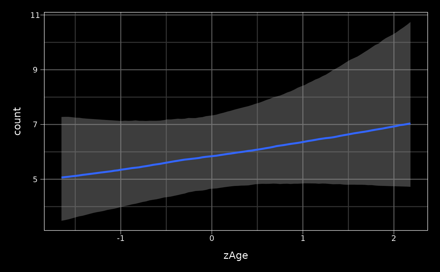
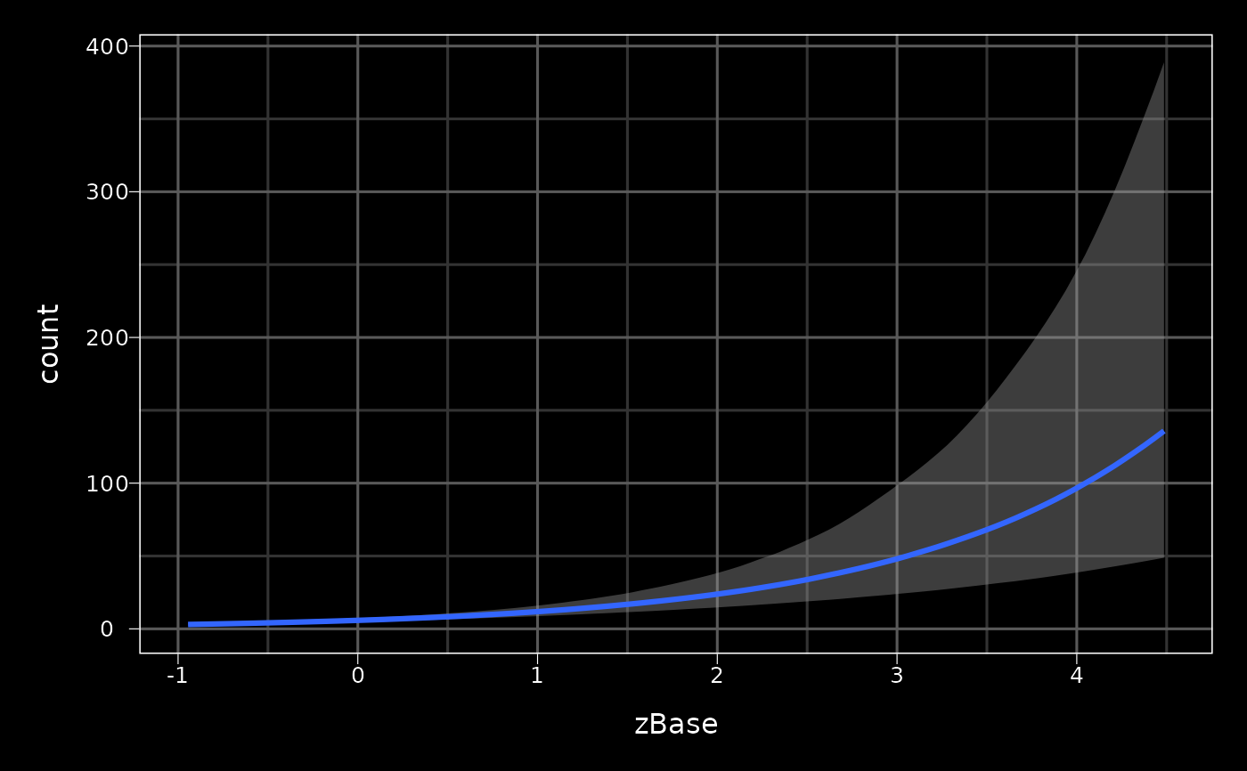
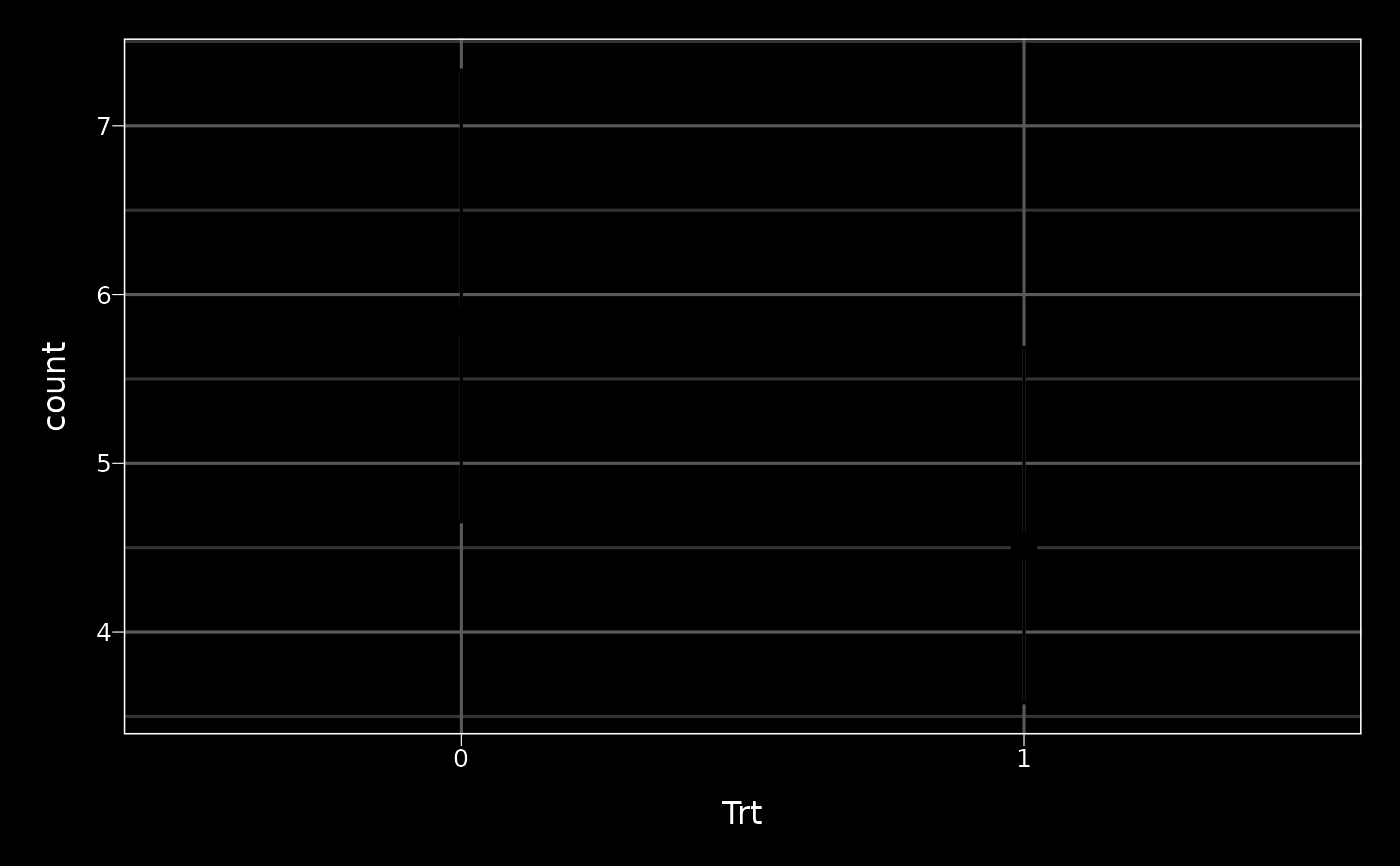
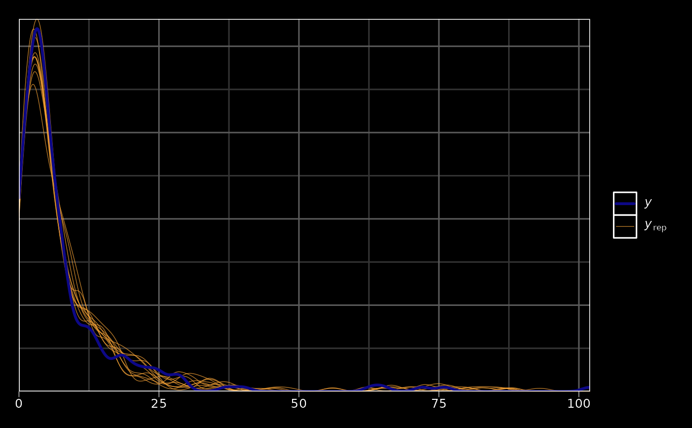
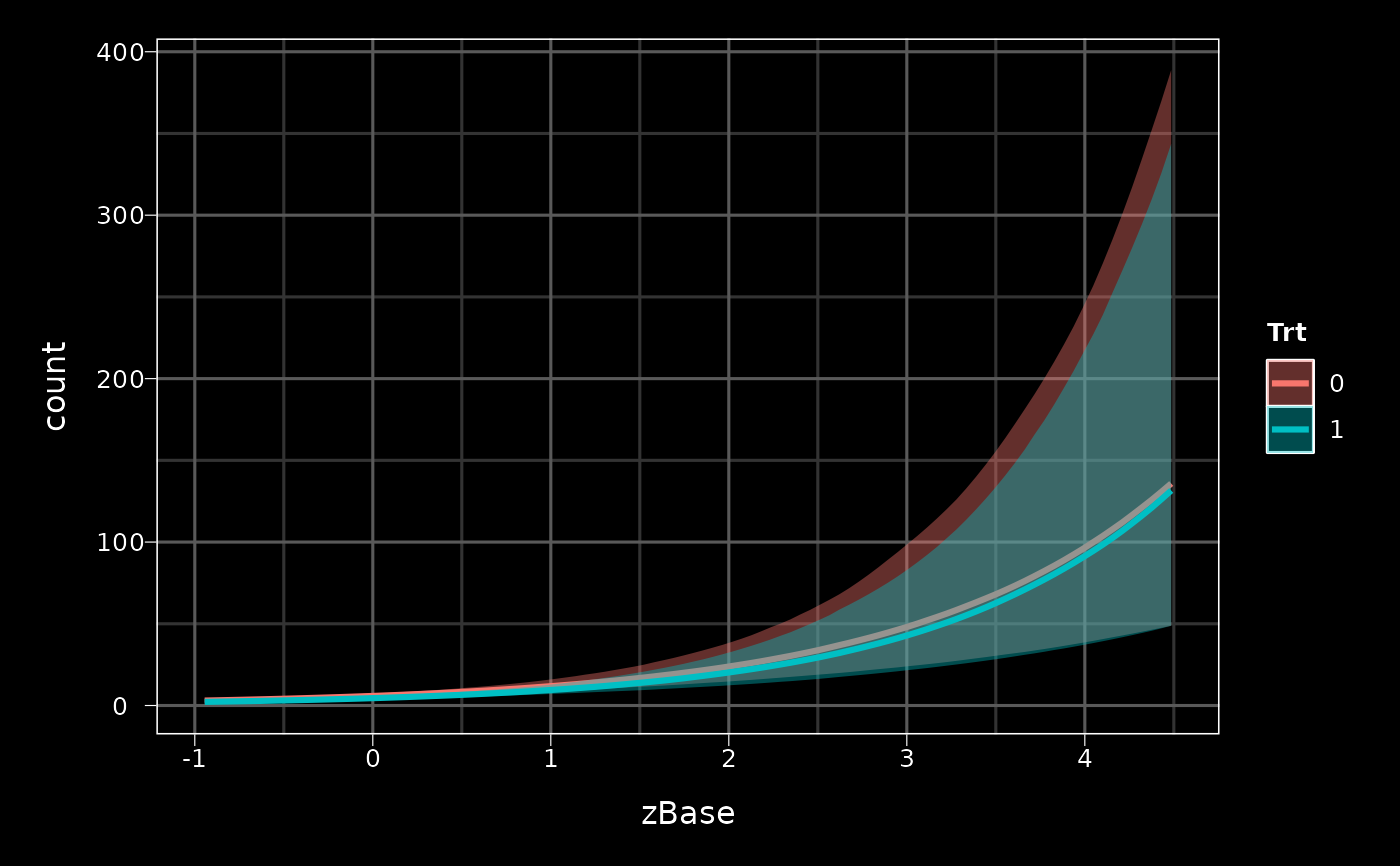 pp_check(fit)
#> Using 10 posterior draws for ppc type 'dens_overlay' by default.
pp_check(fit)
#> Using 10 posterior draws for ppc type 'dens_overlay' by default.
 mcmc_plot(fit, type = "hex", variable = c("b_Intercept", "b_Trt1"))
#> Error in suggested_package("hexbin"): Please install the hexbin package to use this function.
# }
mcmc_plot(fit, type = "hex", variable = c("b_Intercept", "b_Trt1"))
#> Error in suggested_package("hexbin"): Please install the hexbin package to use this function.
# }