
Fit Bayesian generalized (non-)linear multivariate multilevel models using Stan for full Bayesian inference. A wide range of distributions and link functions are supported, allowing users to fit – among others – linear, robust linear, count data, survival, response times, ordinal, zero-inflated, hurdle, extended-support beta regression, and even self-defined mixture models all in a multilevel context. Further modeling options include non-linear and smooth terms, auto-correlation structures, censored data, meta-analytic standard errors, and quite a few more. In addition, all parameters of the response distributions can be predicted in order to perform distributional regression. Prior specifications are flexible and explicitly encourage users to apply prior distributions that actually reflect their beliefs. In addition, model fit can easily be assessed and compared with posterior predictive checks and leave-one-out cross-validation.
Usage
brm(
  formula,
  data,
  family = gaussian(),
  prior = NULL,
  autocor = NULL,
  data2 = NULL,
  cov_ranef = NULL,
  sample_prior = "no",
  sparse = NULL,
  knots = NULL,
  drop_unused_levels = TRUE,
  stanvars = NULL,
  stan_funs = NULL,
  fit = NA,
  save_pars = getOption("brms.save_pars", NULL),
  save_ranef = NULL,
  save_mevars = NULL,
  save_all_pars = NULL,
  init = NULL,
  inits = NULL,
  chains = 4,
  iter = getOption("brms.iter", 2000),
  warmup = floor(iter/2),
  thin = 1,
  cores = getOption("mc.cores", 1),
  threads = getOption("brms.threads", NULL),
  opencl = getOption("brms.opencl", NULL),
  normalize = getOption("brms.normalize", TRUE),
  control = NULL,
  algorithm = getOption("brms.algorithm", "sampling"),
  backend = getOption("brms.backend", "rstan"),
  future = getOption("future", FALSE),
  silent = getOption("brms.silent", 1),
  seed = NA,
  save_model = NULL,
  stan_model_args = list(),
  file = NULL,
  file_compress = TRUE,
  file_refit = getOption("brms.file_refit", "never"),
  empty = FALSE,
  rename = TRUE,
  ...
)
Arguments
- formula
An object of class
formula,brmsformula, ormvbrmsformula(or one that can be coerced to that classes): A symbolic description of the model to be fitted. The details of model specification are explained inbrmsformula.- data
An object of class
data.frame(or one that can be coerced to that class) containing data of all variables used in the model.- family
A description of the response distribution and link function to be used in the model. This can be a family function, a call to a family function or a character string naming the family. Every family function has a
linkargument allowing to specify the link function to be applied on the response variable. If not specified, default links are used. For details of supported families seebrmsfamily. By default, a lineargaussianmodel is applied. In multivariate models,familymight also be a list of families.- prior
One or more
brmspriorobjects created byset_prioror related functions and combined using thecmethod or the+operator. See alsodefault_priorfor more help.- autocor
(Deprecated) An optional
cor_brmsobject describing the correlation structure within the response variable (i.e., the 'autocorrelation'). See the documentation ofcor_brmsfor a description of the available correlation structures. Defaults toNULL, corresponding to no correlations. In multivariate models,autocormight also be a list of autocorrelation structures. It is now recommend to specify autocorrelation terms directly withinformula. Seebrmsformulafor more details.- data2
A named
listof objects containing data, which cannot be passed via argumentdata. Required for some objects used in autocorrelation structures to specify dependency structures as well as for within-group covariance matrices.- cov_ranef
(Deprecated) A list of matrices that are proportional to the (within) covariance structure of the group-level effects. The names of the matrices should correspond to columns in
datathat are used as grouping factors. All levels of the grouping factor should appear as rownames of the corresponding matrix. This argument can be used, among others to model pedigrees and phylogenetic effects. It is now recommended to specify those matrices in the formula interface using thegrand related functions. Seevignette("brms_phylogenetics")for more details.- sample_prior
Indicate if draws from priors should be drawn additionally to the posterior draws. Options are
"no"(the default),"yes", and"only". Among others, these draws can be used to calculate Bayes factors for point hypotheses viahypothesis. Please note that improper priors are not sampled, including the default improper priors used bybrm. Seeset_prioron how to set (proper) priors. Please also note that prior draws for the overall intercept are not obtained by default for technical reasons. Seebrmsformulahow to obtain prior draws for the intercept. Ifsample_prioris set to"only", draws are drawn solely from the priors ignoring the likelihood, which allows among others to generate draws from the prior predictive distribution. In this case, all parameters must have proper priors.- sparse
(Deprecated) Logical; indicates whether the population-level design matrices should be treated as sparse (defaults to
FALSE). For design matrices with many zeros, this can considerably reduce required memory. Sampling speed is currently not improved or even slightly decreased. It is now recommended to use thesparseargument ofbrmsformulaand related functions.- knots
Optional list containing user specified knot values to be used for basis construction of smoothing terms. See
gammfor more details.- drop_unused_levels
Should unused factors levels in the data be dropped? Defaults to
TRUE.- stanvars
An optional
stanvarsobject generated by functionstanvarto define additional variables for use in Stan's program blocks.- stan_funs
(Deprecated) An optional character string containing self-defined Stan functions, which will be included in the functions block of the generated Stan code. It is now recommended to use the
stanvarsargument for this purpose instead.- fit
An instance of S3 class
brmsfitderived from a previous fit; defaults toNA. Iffitis of classbrmsfit, the compiled model associated with the fitted result is re-used and all arguments modifying the model code or data are ignored. It is not recommended to use this argument directly, but to call theupdatemethod, instead.- save_pars
An object generated by
save_parscontrolling which parameters should be saved in the model. The argument has no impact on the model fitting itself.- save_ranef
(Deprecated) A flag to indicate if group-level effects for each level of the grouping factor(s) should be saved (default is
TRUE). Set toFALSEto save memory. The argument has no impact on the model fitting itself.- save_mevars
(Deprecated) A flag to indicate if draws of latent noise-free variables obtained by using
meandmiterms should be saved (default isFALSE). Saving these draws allows to better use methods such aspredictwith the latent variables but leads to very large R objects even for models of moderate size and complexity.- save_all_pars
(Deprecated) A flag to indicate if draws from all variables defined in Stan's
parametersblock should be saved (default isFALSE). Saving these draws is required in order to apply the methodsbridge_sampler,bayes_factor, andpost_prob. Can be set globally for the current R session via the"brms.save_pars"option (seeoptions).- init
Initial values for the sampler. If
NULL(the default) or"random", Stan will randomly generate initial values for parameters in a reasonable range. If0, all parameters are initialized to zero on the unconstrained space. This option is sometimes useful for certain families, as it happens that default random initial values cause draws to be essentially constant. Generally, settinginit = 0is worth a try, if chains do not initialize or behave well. Alternatively,initcan be a list of lists containing the initial values, or a function (or function name) generating initial values. The latter options are mainly implemented for internal testing but are available to users if necessary. If specifying initial values using a list or a function then currently the parameter names must correspond to the names used in the generated Stan code (not the names used in R). For more details on specifying initial values you can consult the documentation of the selectedbackend.- inits
(Deprecated) Alias of
init.- chains
Number of Markov chains (defaults to 4).
- iter
Number of total iterations per chain (including warmup; defaults to 2000). Can be set globally for the current R session via the
"brms.iter"option (seeoptions).- warmup
A positive integer specifying number of warmup (aka burnin) iterations. This also specifies the number of iterations used for stepsize adaptation, so warmup draws should not be used for inference. The number of warmup should not be larger than
iterand the default isiter/2.- thin
Thinning rate. Must be a positive integer. Set
thin > 1to save memory and computation time ifiteris large.- cores
Number of cores to use when executing the chains in parallel, which defaults to 1 but we recommend setting the
mc.coresoption to be as many processors as the hardware and RAM allow (up to the number of chains). For non-Windows OS in non-interactive R sessions, forking is used instead of PSOCK clusters.- threads
Number of threads to use in within-chain parallelization. For more control over the threading process,
threadsmay also be abrmsthreadsobject created bythreading. Within-chain parallelization is experimental! We recommend its use only if you are experienced with Stan'sreduce_sumfunction and have a slow running model that cannot be sped up by any other means. Can be set globally for the current R session via the"brms.threads"option (seeoptions).- opencl
The platform and device IDs of the OpenCL device to use for fitting using GPU support. If you don't know the IDs of your OpenCL device,
c(0,0)is most likely what you need. For more details, seeopencl. Can be set globally for the current R session via the"brms.opencl"option- normalize
Logical. Indicates whether normalization constants should be included in the Stan code (defaults to
TRUE). Setting it toFALSErequires Stan version >= 2.25 to work. IfFALSE, sampling efficiency may be increased but some post processing functions such asbridge_samplerwill not be available. Can be controlled globally for the current R session via the `brms.normalize` option.- control
A named
listof parameters to control the sampler's behavior. It defaults toNULLso all the default values are used. The most important control parameters are discussed in the 'Details' section below. For a comprehensive overview seestan.- algorithm
Character string naming the estimation approach to use. Options are
"sampling"for MCMC (the default),"meanfield"for variational inference with independent normal distributions,"fullrank"for variational inference with a multivariate normal distribution,"pathfinder"for the pathfinder algorithm,"laplace"for the laplace approximation, or"fixed_param"for sampling from fixed parameter values. Can be set globally for the current R session via the"brms.algorithm"option (seeoptions).- backend
Character string naming the package to use as the backend for fitting the Stan model. Options are
"rstan"(the default) or"cmdstanr". Can be set globally for the current R session via the"brms.backend"option (seeoptions). Details on the rstan and cmdstanr packages are available at https://mc-stan.org/rstan/ and https://mc-stan.org/cmdstanr/, respectively. Additionally a"mock"backend is available to make testing brms and packages that depend on it easier. The"mock"backend does not actually do any fitting, it only checks the generated Stan code for correctness and then returns whatever is passed in an additionalmock_fitargument as the result of the fit.- future
Logical; If
TRUE, the future package is used for parallel execution of the chains and argumentcoreswill be ignored. Can be set globally for the current R session via the"future"option. The execution type is controlled viaplan(see the examples section below).- silent
Verbosity level between
0and2. If1(the default), most of the informational messages of compiler and sampler are suppressed. If2, even more messages are suppressed. The actual sampling progress is still printed. Setrefresh = 0to turn this off as well. If usingbackend = "rstan"you can also setopen_progress = FALSEto prevent opening additional progress bars. Can be set globally for the current R session via the"brms.silent"option (seeoptions).- seed
The seed for random number generation to make results reproducible. If
NA(the default), Stan will set the seed randomly.- save_model
Either
NULLor a character string. In the latter case, the model's Stan code is saved viacatin a text file named after the string supplied insave_model.- stan_model_args
A
listof further arguments passed torstan::stan_modelforbackend = "rstan"or tocmdstanr::cmdstan_modelforbackend = "cmdstanr", which allows to change how models are compiled.- file
Either
NULLor a character string. In the latter case, the fitted model object is saved viasaveRDSin a file named after the string supplied infile. The.rdsextension is added automatically. If the file already exists,brmwill load and return the saved model object instead of refitting the model. Unless you specify thefile_refitargument as well, the existing files won't be overwritten, you have to manually remove the file in order to refit and save the model under an existing file name. The file name is stored in thebrmsfitobject for later usage.- file_compress
Logical or a character string, specifying one of the compression algorithms supported by
saveRDS. If thefileargument is provided, this compression will be used when saving the fitted model object.- file_refit
Modifies when the fit stored via the
fileargument is re-used. Can be set globally for the current R session via the"brms.file_refit"option (seeoptions). For"never"(default) the fit is always loaded if it exists and fitting is skipped. For"always"the model is always refitted. If set to"on_change", brms will refit the model if model, data or algorithm as passed to Stan differ from what is stored in the file. This also covers changes in priors,sample_prior,stanvars, covariance structure, etc. If you believe there was a false positive, you can usebrmsfit_needs_refitto see why refit is deemed necessary. Refit will not be triggered for changes in additional parameters of the fit (e.g., initial values, number of iterations, control arguments, ...). A known limitation is that a refit will be triggered if within-chain parallelization is switched on/off.- empty
Logical. If
TRUE, the Stan model is not created and compiled and the corresponding'fit'slot of thebrmsfitobject will be empty. This is useful if you have estimated a brms-created Stan model outside of brms and want to feed it back into the package.- rename
For internal use only.
- ...
Further arguments passed to Stan. For
backend = "rstan"the arguments are passed tosamplingorvb. Forbackend = "cmdstanr"the arguments are passed to thecmdstanr::sampleorcmdstanr::variationalmethod.
Value
An object of class brmsfit, which contains the posterior
draws along with many other useful information about the model. Use
methods(class = "brmsfit") for an overview on available methods.
Details
Fit a generalized (non-)linear multivariate multilevel model via
full Bayesian inference using Stan. A general overview is provided in the
vignettes vignette("brms_overview") and
vignette("brms_multilevel"). For a full list of available vignettes
see vignette(package = "brms").
Formula syntax of brms models
Details of the formula syntax applied in brms can be found in
brmsformula.
Families and link functions
Details of families supported by brms can be found in
brmsfamily.
Prior distributions
Priors should be specified using the
set_prior function. Its documentation
contains detailed information on how to correctly specify priors. To find
out on which parameters or parameter classes priors can be defined, use
default_prior. Default priors are chosen to be
non or very weakly informative so that their influence on the results will
be negligible and you usually don't have to worry about them. However,
after getting more familiar with Bayesian statistics, I recommend you to
start thinking about reasonable informative priors for your model
parameters: Nearly always, there is at least some prior information
available that can be used to improve your inference.
Adjusting the sampling behavior of Stan
In addition to choosing the number of iterations, warmup draws, and
chains, users can control the behavior of the NUTS sampler, by using the
control argument. The most important reason to use control is
to decrease (or eliminate at best) the number of divergent transitions that
cause a bias in the obtained posterior draws. Whenever you see the
warning "There were x divergent transitions after warmup." you should
really think about increasing adapt_delta. To do this, write
control = list(adapt_delta = <x>), where <x> should usually
be value between 0.8 (current default) and 1. Increasing
adapt_delta will slow down the sampler but will decrease the number
of divergent transitions threatening the validity of your posterior
draws.
Another problem arises when the depth of the tree being evaluated in each
iteration is exceeded. This is less common than having divergent
transitions, but may also bias the posterior draws. When it happens,
Stan will throw out a warning suggesting to increase
max_treedepth, which can be accomplished by writing control =
list(max_treedepth = <x>) with a positive integer <x> that should
usually be larger than the current default of 10. For more details
on the control argument see stan.
Parallelization with multiple CPU cores
brms can make use of multiple CPU cores in parallel to speed
up computations in various ways. For efficient use of the
available resources it is recommended to only use parallelism to
an extend such that the available physical CPUs are not
oversubscribed. For example, when you have 8 CPU cores locally
available, then you may consider to run 4 chains with 2 threads
per chain for best performance if you happen to just run a single
model. In case you run a simulation study which requires to run
many times a given model, then neither chain nor within-chain
parallelization is advisable as the computational resources are
already exhausted by the simulation study and any further
parallelization beyond the simulation study itself will in fact
slow down the overall runtime. Please be aware that for
historical reasons the nomenclature of the arguments is possibly
confusing. The cores argument refers to running different
chains in parallel and the within-chain parallelization will
allocate for each chain as many threads as requested. The
requested threads therefore increase the use of overall CPUs in a
multiplicative way.
For more advanced parallelization (including beyond single model
fits), brms also integrates with the future
package. Importantly, this enables seamless integration with the
mirai parallelization framework through the use of the
future.mirai adapter. With mirai local and remote
machines can be used in a fully transparent manner to the
user. This includes the possibility to use large number of remote
machines running in the context of a computer cluster, which are
managed with queuing systems. Please refer to the section on
distributed computing of
mirai::daemons.
References
Paul-Christian Buerkner (2017). brms: An R Package for Bayesian Multilevel
Models Using Stan. Journal of Statistical Software, 80(1), 1-28.
doi:10.18637/jss.v080.i01
Paul-Christian Buerkner (2018). Advanced Bayesian Multilevel Modeling
with the R Package brms. The R Journal. 10(1), 395–411.
doi:10.32614/RJ-2018-017
Author
Paul-Christian Buerkner paul.buerkner@gmail.com
Examples
# \dontrun{
# Poisson regression for the number of seizures in epileptic patients
fit1 <- brm(
count ~ zBase * Trt + (1|patient),
data = epilepsy, family = poisson(),
prior = prior(normal(0, 10), class = b) +
prior(cauchy(0, 2), class = sd)
)
#> Compiling Stan program...
#> Start sampling
#>
#> SAMPLING FOR MODEL 'anon_model' NOW (CHAIN 1).
#> Chain 1:
#> Chain 1: Gradient evaluation took 3.2e-05 seconds
#> Chain 1: 1000 transitions using 10 leapfrog steps per transition would take 0.32 seconds.
#> Chain 1: Adjust your expectations accordingly!
#> Chain 1:
#> Chain 1:
#> Chain 1: Iteration: 1 / 2000 [ 0%] (Warmup)
#> Chain 1: Iteration: 200 / 2000 [ 10%] (Warmup)
#> Chain 1: Iteration: 400 / 2000 [ 20%] (Warmup)
#> Chain 1: Iteration: 600 / 2000 [ 30%] (Warmup)
#> Chain 1: Iteration: 800 / 2000 [ 40%] (Warmup)
#> Chain 1: Iteration: 1000 / 2000 [ 50%] (Warmup)
#> Chain 1: Iteration: 1001 / 2000 [ 50%] (Sampling)
#> Chain 1: Iteration: 1200 / 2000 [ 60%] (Sampling)
#> Chain 1: Iteration: 1400 / 2000 [ 70%] (Sampling)
#> Chain 1: Iteration: 1600 / 2000 [ 80%] (Sampling)
#> Chain 1: Iteration: 1800 / 2000 [ 90%] (Sampling)
#> Chain 1: Iteration: 2000 / 2000 [100%] (Sampling)
#> Chain 1:
#> Chain 1: Elapsed Time: 2.13 seconds (Warm-up)
#> Chain 1: 1.5 seconds (Sampling)
#> Chain 1: 3.63 seconds (Total)
#> Chain 1:
#>
#> SAMPLING FOR MODEL 'anon_model' NOW (CHAIN 2).
#> Chain 2:
#> Chain 2: Gradient evaluation took 2.8e-05 seconds
#> Chain 2: 1000 transitions using 10 leapfrog steps per transition would take 0.28 seconds.
#> Chain 2: Adjust your expectations accordingly!
#> Chain 2:
#> Chain 2:
#> Chain 2: Iteration: 1 / 2000 [ 0%] (Warmup)
#> Chain 2: Iteration: 200 / 2000 [ 10%] (Warmup)
#> Chain 2: Iteration: 400 / 2000 [ 20%] (Warmup)
#> Chain 2: Iteration: 600 / 2000 [ 30%] (Warmup)
#> Chain 2: Iteration: 800 / 2000 [ 40%] (Warmup)
#> Chain 2: Iteration: 1000 / 2000 [ 50%] (Warmup)
#> Chain 2: Iteration: 1001 / 2000 [ 50%] (Sampling)
#> Chain 2: Iteration: 1200 / 2000 [ 60%] (Sampling)
#> Chain 2: Iteration: 1400 / 2000 [ 70%] (Sampling)
#> Chain 2: Iteration: 1600 / 2000 [ 80%] (Sampling)
#> Chain 2: Iteration: 1800 / 2000 [ 90%] (Sampling)
#> Chain 2: Iteration: 2000 / 2000 [100%] (Sampling)
#> Chain 2:
#> Chain 2: Elapsed Time: 2.131 seconds (Warm-up)
#> Chain 2: 1.477 seconds (Sampling)
#> Chain 2: 3.608 seconds (Total)
#> Chain 2:
#>
#> SAMPLING FOR MODEL 'anon_model' NOW (CHAIN 3).
#> Chain 3:
#> Chain 3: Gradient evaluation took 2.6e-05 seconds
#> Chain 3: 1000 transitions using 10 leapfrog steps per transition would take 0.26 seconds.
#> Chain 3: Adjust your expectations accordingly!
#> Chain 3:
#> Chain 3:
#> Chain 3: Iteration: 1 / 2000 [ 0%] (Warmup)
#> Chain 3: Iteration: 200 / 2000 [ 10%] (Warmup)
#> Chain 3: Iteration: 400 / 2000 [ 20%] (Warmup)
#> Chain 3: Iteration: 600 / 2000 [ 30%] (Warmup)
#> Chain 3: Iteration: 800 / 2000 [ 40%] (Warmup)
#> Chain 3: Iteration: 1000 / 2000 [ 50%] (Warmup)
#> Chain 3: Iteration: 1001 / 2000 [ 50%] (Sampling)
#> Chain 3: Iteration: 1200 / 2000 [ 60%] (Sampling)
#> Chain 3: Iteration: 1400 / 2000 [ 70%] (Sampling)
#> Chain 3: Iteration: 1600 / 2000 [ 80%] (Sampling)
#> Chain 3: Iteration: 1800 / 2000 [ 90%] (Sampling)
#> Chain 3: Iteration: 2000 / 2000 [100%] (Sampling)
#> Chain 3:
#> Chain 3: Elapsed Time: 1.852 seconds (Warm-up)
#> Chain 3: 1.527 seconds (Sampling)
#> Chain 3: 3.379 seconds (Total)
#> Chain 3:
#>
#> SAMPLING FOR MODEL 'anon_model' NOW (CHAIN 4).
#> Chain 4:
#> Chain 4: Gradient evaluation took 2.5e-05 seconds
#> Chain 4: 1000 transitions using 10 leapfrog steps per transition would take 0.25 seconds.
#> Chain 4: Adjust your expectations accordingly!
#> Chain 4:
#> Chain 4:
#> Chain 4: Iteration: 1 / 2000 [ 0%] (Warmup)
#> Chain 4: Iteration: 200 / 2000 [ 10%] (Warmup)
#> Chain 4: Iteration: 400 / 2000 [ 20%] (Warmup)
#> Chain 4: Iteration: 600 / 2000 [ 30%] (Warmup)
#> Chain 4: Iteration: 800 / 2000 [ 40%] (Warmup)
#> Chain 4: Iteration: 1000 / 2000 [ 50%] (Warmup)
#> Chain 4: Iteration: 1001 / 2000 [ 50%] (Sampling)
#> Chain 4: Iteration: 1200 / 2000 [ 60%] (Sampling)
#> Chain 4: Iteration: 1400 / 2000 [ 70%] (Sampling)
#> Chain 4: Iteration: 1600 / 2000 [ 80%] (Sampling)
#> Chain 4: Iteration: 1800 / 2000 [ 90%] (Sampling)
#> Chain 4: Iteration: 2000 / 2000 [100%] (Sampling)
#> Chain 4:
#> Chain 4: Elapsed Time: 2.064 seconds (Warm-up)
#> Chain 4: 1.662 seconds (Sampling)
#> Chain 4: 3.726 seconds (Total)
#> Chain 4:
# generate a summary of the results
summary(fit1)
#> Family: poisson
#> Links: mu = log
#> Formula: count ~ zBase * Trt + (1 | patient)
#> Data: epilepsy (Number of observations: 236)
#> Draws: 4 chains, each with iter = 2000; warmup = 1000; thin = 1;
#> total post-warmup draws = 4000
#>
#> Multilevel Hyperparameters:
#> ~patient (Number of levels: 59)
#> Estimate Est.Error l-95% CI u-95% CI Rhat Bulk_ESS Tail_ESS
#> sd(Intercept) 0.59 0.07 0.46 0.74 1.01 606 1109
#>
#> Regression Coefficients:
#> Estimate Est.Error l-95% CI u-95% CI Rhat Bulk_ESS Tail_ESS
#> Intercept 1.79 0.12 1.55 2.03 1.00 682 1268
#> zBase 0.70 0.12 0.46 0.95 1.00 720 968
#> Trt1 -0.29 0.18 -0.63 0.05 1.01 548 828
#> zBase:Trt1 0.02 0.17 -0.30 0.36 1.01 720 1258
#>
#> Draws were sampled using sampling(NUTS). For each parameter, Bulk_ESS
#> and Tail_ESS are effective sample size measures, and Rhat is the potential
#> scale reduction factor on split chains (at convergence, Rhat = 1).
# plot the MCMC chains as well as the posterior distributions
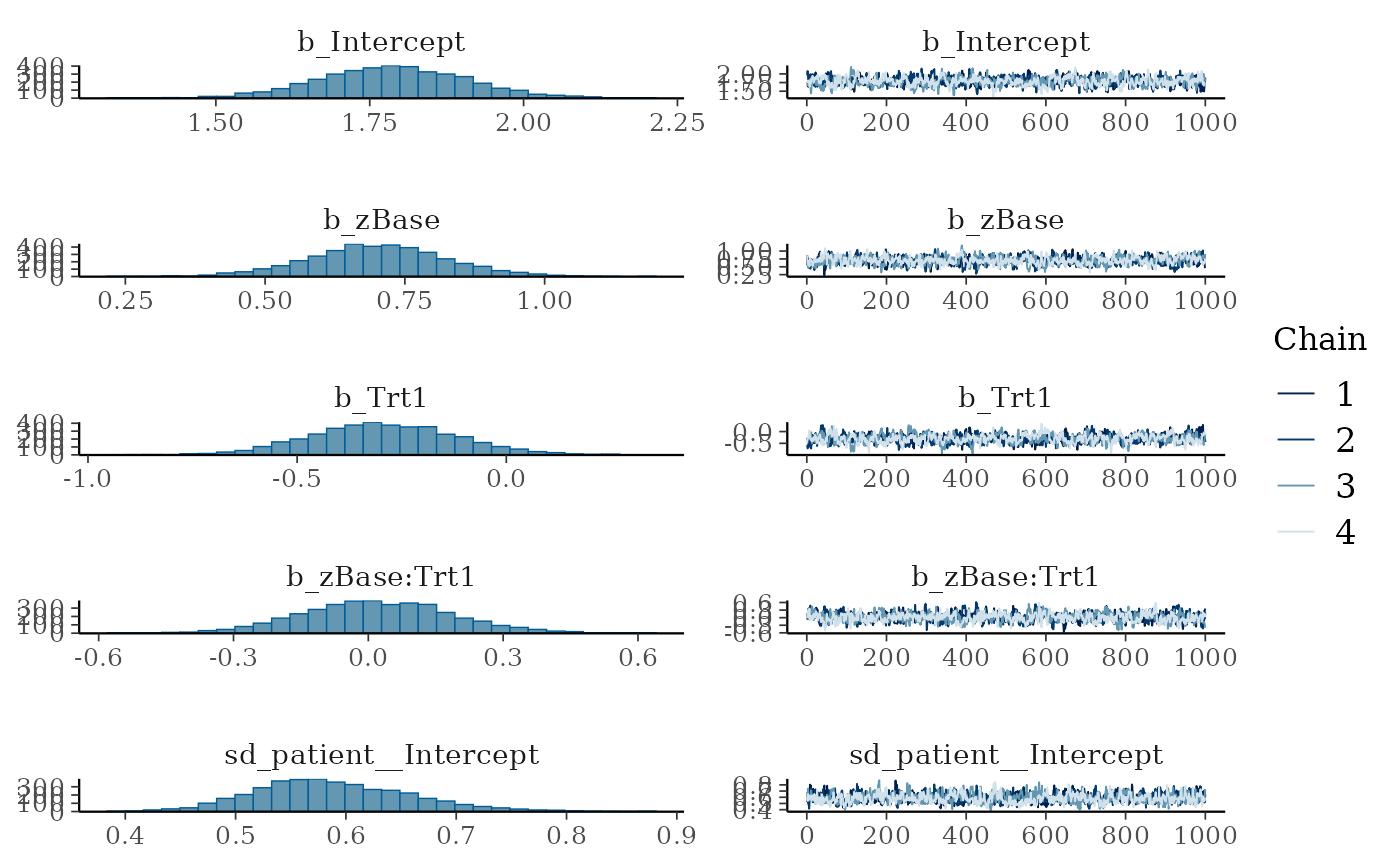
plot(fit1)
 # predict responses based on the fitted model
head(predict(fit1))
#> Estimate Est.Error Q2.5 Q97.5
#> [1,] 3.48525 1.995063 0 8
#> [2,] 3.54450 2.034712 0 8
#> [3,] 2.80625 1.867105 0 7
#> [4,] 3.25575 1.939789 0 8
#> [5,] 13.84325 4.151565 6 23
#> [6,] 5.46925 2.607826 1 11
# plot conditional effects for each predictor
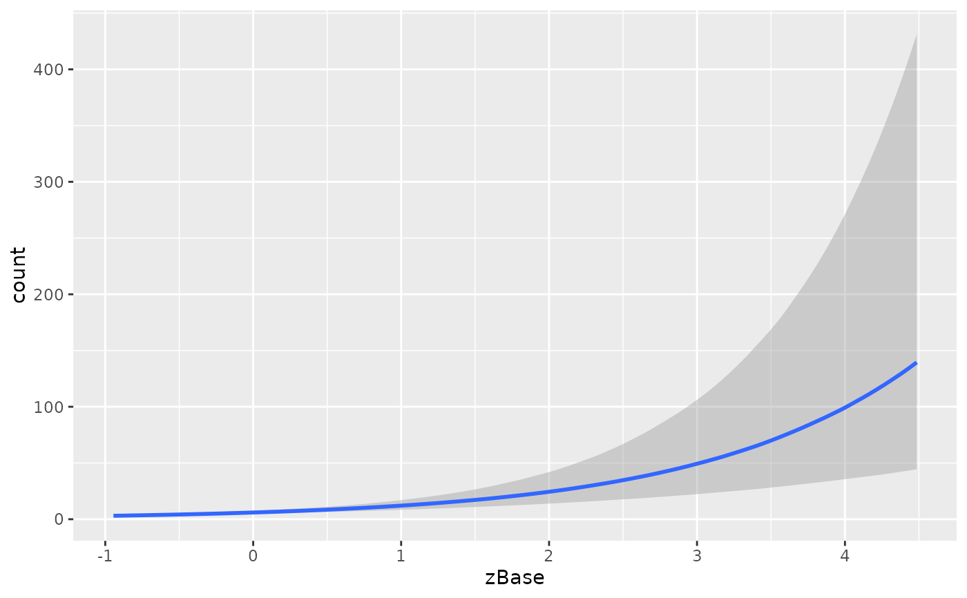
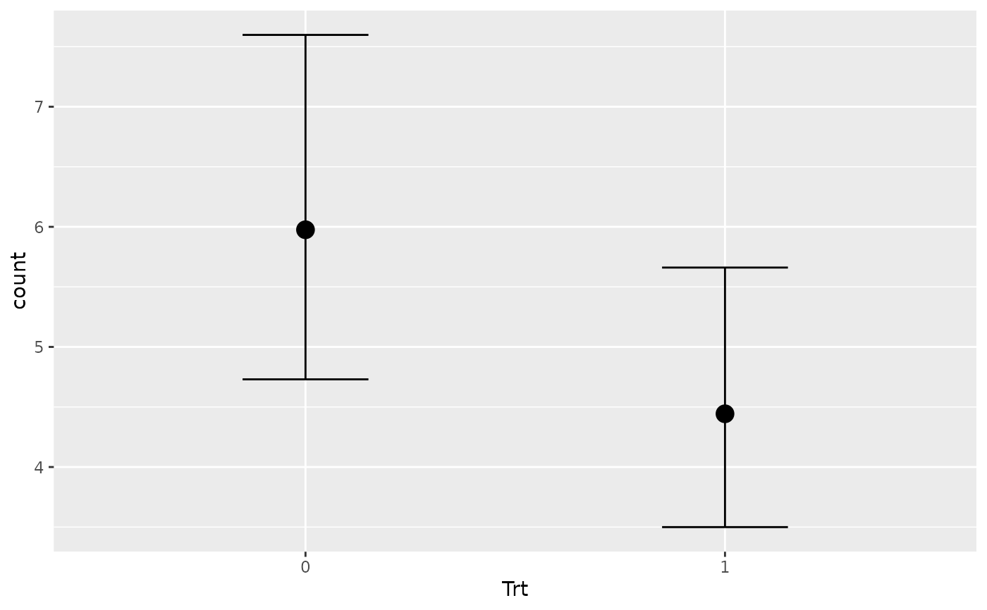
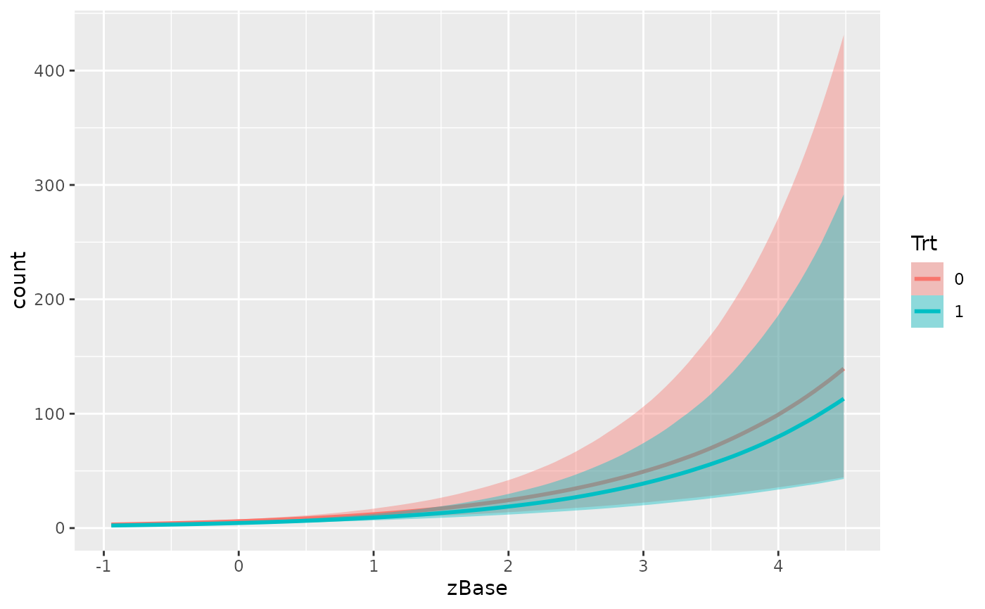
plot(conditional_effects(fit1), ask = FALSE)
# predict responses based on the fitted model
head(predict(fit1))
#> Estimate Est.Error Q2.5 Q97.5
#> [1,] 3.48525 1.995063 0 8
#> [2,] 3.54450 2.034712 0 8
#> [3,] 2.80625 1.867105 0 7
#> [4,] 3.25575 1.939789 0 8
#> [5,] 13.84325 4.151565 6 23
#> [6,] 5.46925 2.607826 1 11
# plot conditional effects for each predictor
plot(conditional_effects(fit1), ask = FALSE)
 # investigate model fit
loo(fit1)
#> Warning: Found 8 observations with a pareto_k > 0.7 in model 'fit1'. We recommend to set 'moment_match = TRUE' in order to perform moment matching for problematic observations.
#>
#> Computed from 4000 by 236 log-likelihood matrix.
#>
#> Estimate SE
#> elpd_loo -670.7 36.3
#> p_loo 93.3 14.0
#> looic 1341.3 72.7
#> ------
#> MCSE of elpd_loo is NA.
#> MCSE and ESS estimates assume MCMC draws (r_eff in [0.3, 2.6]).
#>
#> Pareto k diagnostic values:
#> Count Pct. Min. ESS
#> (-Inf, 0.7] (good) 228 96.6% 160
#> (0.7, 1] (bad) 6 2.5% <NA>
#> (1, Inf) (very bad) 2 0.8% <NA>
#> See help('pareto-k-diagnostic') for details.
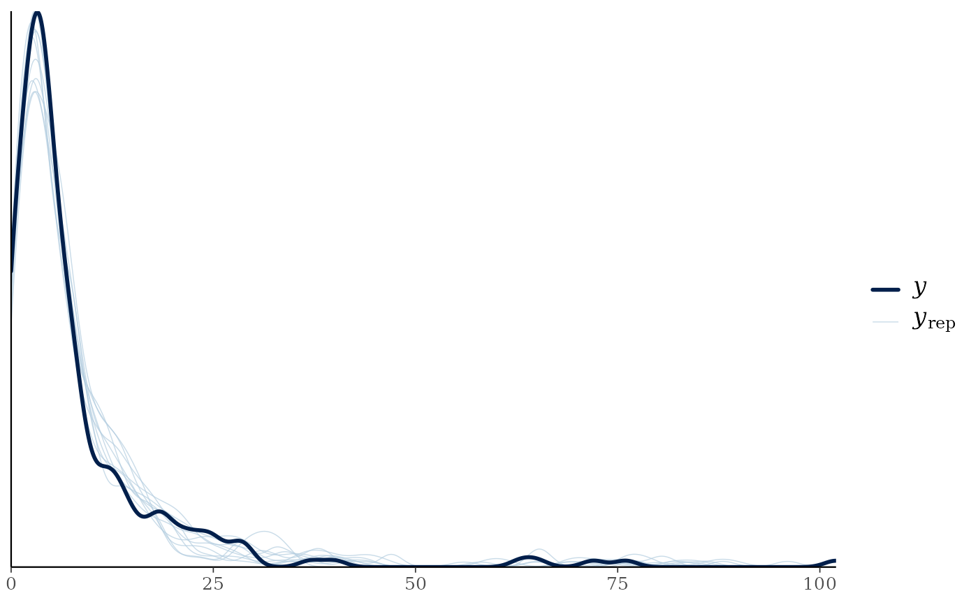
pp_check(fit1)
#> Using 10 posterior draws for ppc type 'dens_overlay' by default.
# investigate model fit
loo(fit1)
#> Warning: Found 8 observations with a pareto_k > 0.7 in model 'fit1'. We recommend to set 'moment_match = TRUE' in order to perform moment matching for problematic observations.
#>
#> Computed from 4000 by 236 log-likelihood matrix.
#>
#> Estimate SE
#> elpd_loo -670.7 36.3
#> p_loo 93.3 14.0
#> looic 1341.3 72.7
#> ------
#> MCSE of elpd_loo is NA.
#> MCSE and ESS estimates assume MCMC draws (r_eff in [0.3, 2.6]).
#>
#> Pareto k diagnostic values:
#> Count Pct. Min. ESS
#> (-Inf, 0.7] (good) 228 96.6% 160
#> (0.7, 1] (bad) 6 2.5% <NA>
#> (1, Inf) (very bad) 2 0.8% <NA>
#> See help('pareto-k-diagnostic') for details.
pp_check(fit1)
#> Using 10 posterior draws for ppc type 'dens_overlay' by default.
 # Ordinal regression modeling patient's rating of inhaler instructions
# category specific effects are estimated for variable 'treat'
fit2 <- brm(rating ~ period + carry + cs(treat),
data = inhaler, family = sratio("logit"),
prior = set_prior("normal(0,5)"), chains = 2)
#> Compiling Stan program...
#> Start sampling
#>
#> SAMPLING FOR MODEL 'anon_model' NOW (CHAIN 1).
#> Chain 1:
#> Chain 1: Gradient evaluation took 0.000267 seconds
#> Chain 1: 1000 transitions using 10 leapfrog steps per transition would take 2.67 seconds.
#> Chain 1: Adjust your expectations accordingly!
#> Chain 1:
#> Chain 1:
#> Chain 1: Iteration: 1 / 2000 [ 0%] (Warmup)
#> Chain 1: Iteration: 200 / 2000 [ 10%] (Warmup)
#> Chain 1: Iteration: 400 / 2000 [ 20%] (Warmup)
#> Chain 1: Iteration: 600 / 2000 [ 30%] (Warmup)
#> Chain 1: Iteration: 800 / 2000 [ 40%] (Warmup)
#> Chain 1: Iteration: 1000 / 2000 [ 50%] (Warmup)
#> Chain 1: Iteration: 1001 / 2000 [ 50%] (Sampling)
#> Chain 1: Iteration: 1200 / 2000 [ 60%] (Sampling)
#> Chain 1: Iteration: 1400 / 2000 [ 70%] (Sampling)
#> Chain 1: Iteration: 1600 / 2000 [ 80%] (Sampling)
#> Chain 1: Iteration: 1800 / 2000 [ 90%] (Sampling)
#> Chain 1: Iteration: 2000 / 2000 [100%] (Sampling)
#> Chain 1:
#> Chain 1: Elapsed Time: 2.737 seconds (Warm-up)
#> Chain 1: 2.648 seconds (Sampling)
#> Chain 1: 5.385 seconds (Total)
#> Chain 1:
#>
#> SAMPLING FOR MODEL 'anon_model' NOW (CHAIN 2).
#> Chain 2:
#> Chain 2: Gradient evaluation took 0.000241 seconds
#> Chain 2: 1000 transitions using 10 leapfrog steps per transition would take 2.41 seconds.
#> Chain 2: Adjust your expectations accordingly!
#> Chain 2:
#> Chain 2:
#> Chain 2: Iteration: 1 / 2000 [ 0%] (Warmup)
#> Chain 2: Iteration: 200 / 2000 [ 10%] (Warmup)
#> Chain 2: Iteration: 400 / 2000 [ 20%] (Warmup)
#> Chain 2: Iteration: 600 / 2000 [ 30%] (Warmup)
#> Chain 2: Iteration: 800 / 2000 [ 40%] (Warmup)
#> Chain 2: Iteration: 1000 / 2000 [ 50%] (Warmup)
#> Chain 2: Iteration: 1001 / 2000 [ 50%] (Sampling)
#> Chain 2: Iteration: 1200 / 2000 [ 60%] (Sampling)
#> Chain 2: Iteration: 1400 / 2000 [ 70%] (Sampling)
#> Chain 2: Iteration: 1600 / 2000 [ 80%] (Sampling)
#> Chain 2: Iteration: 1800 / 2000 [ 90%] (Sampling)
#> Chain 2: Iteration: 2000 / 2000 [100%] (Sampling)
#> Chain 2:
#> Chain 2: Elapsed Time: 2.848 seconds (Warm-up)
#> Chain 2: 2.468 seconds (Sampling)
#> Chain 2: 5.316 seconds (Total)
#> Chain 2:
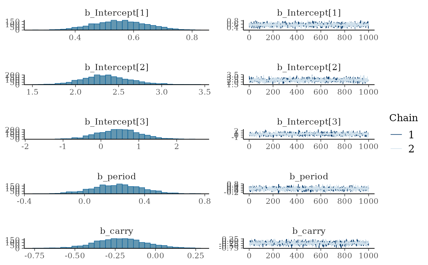
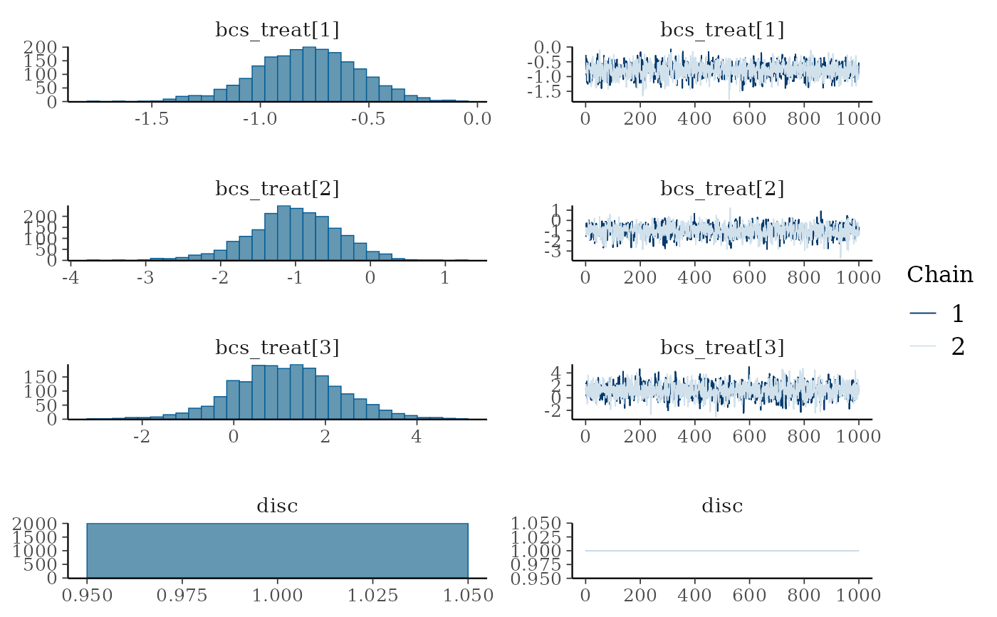
summary(fit2)
#> Family: sratio
#> Links: mu = logit
#> Formula: rating ~ period + carry + cs(treat)
#> Data: inhaler (Number of observations: 572)
#> Draws: 2 chains, each with iter = 2000; warmup = 1000; thin = 1;
#> total post-warmup draws = 2000
#>
#> Regression Coefficients:
#> Estimate Est.Error l-95% CI u-95% CI Rhat Bulk_ESS Tail_ESS
#> Intercept[1] 0.55 0.09 0.38 0.73 1.00 2298 1517
#> Intercept[2] 2.36 0.29 1.83 2.98 1.00 1947 1213
#> Intercept[3] 0.48 0.58 -0.67 1.64 1.00 1892 1328
#> period 0.22 0.17 -0.11 0.55 1.00 2497 1272
#> carry -0.22 0.16 -0.53 0.12 1.00 1675 1684
#> treat[1] -0.78 0.24 -1.28 -0.34 1.00 1912 1650
#> treat[2] -1.03 0.59 -2.29 0.07 1.00 1592 1500
#> treat[3] 1.15 1.15 -1.14 3.44 1.00 1594 1100
#>
#> Further Distributional Parameters:
#> Estimate Est.Error l-95% CI u-95% CI Rhat Bulk_ESS Tail_ESS
#> disc 1.00 0.00 1.00 1.00 NA NA NA
#>
#> Draws were sampled using sampling(NUTS). For each parameter, Bulk_ESS
#> and Tail_ESS are effective sample size measures, and Rhat is the potential
#> scale reduction factor on split chains (at convergence, Rhat = 1).
plot(fit2, ask = FALSE)
# Ordinal regression modeling patient's rating of inhaler instructions
# category specific effects are estimated for variable 'treat'
fit2 <- brm(rating ~ period + carry + cs(treat),
data = inhaler, family = sratio("logit"),
prior = set_prior("normal(0,5)"), chains = 2)
#> Compiling Stan program...
#> Start sampling
#>
#> SAMPLING FOR MODEL 'anon_model' NOW (CHAIN 1).
#> Chain 1:
#> Chain 1: Gradient evaluation took 0.000267 seconds
#> Chain 1: 1000 transitions using 10 leapfrog steps per transition would take 2.67 seconds.
#> Chain 1: Adjust your expectations accordingly!
#> Chain 1:
#> Chain 1:
#> Chain 1: Iteration: 1 / 2000 [ 0%] (Warmup)
#> Chain 1: Iteration: 200 / 2000 [ 10%] (Warmup)
#> Chain 1: Iteration: 400 / 2000 [ 20%] (Warmup)
#> Chain 1: Iteration: 600 / 2000 [ 30%] (Warmup)
#> Chain 1: Iteration: 800 / 2000 [ 40%] (Warmup)
#> Chain 1: Iteration: 1000 / 2000 [ 50%] (Warmup)
#> Chain 1: Iteration: 1001 / 2000 [ 50%] (Sampling)
#> Chain 1: Iteration: 1200 / 2000 [ 60%] (Sampling)
#> Chain 1: Iteration: 1400 / 2000 [ 70%] (Sampling)
#> Chain 1: Iteration: 1600 / 2000 [ 80%] (Sampling)
#> Chain 1: Iteration: 1800 / 2000 [ 90%] (Sampling)
#> Chain 1: Iteration: 2000 / 2000 [100%] (Sampling)
#> Chain 1:
#> Chain 1: Elapsed Time: 2.737 seconds (Warm-up)
#> Chain 1: 2.648 seconds (Sampling)
#> Chain 1: 5.385 seconds (Total)
#> Chain 1:
#>
#> SAMPLING FOR MODEL 'anon_model' NOW (CHAIN 2).
#> Chain 2:
#> Chain 2: Gradient evaluation took 0.000241 seconds
#> Chain 2: 1000 transitions using 10 leapfrog steps per transition would take 2.41 seconds.
#> Chain 2: Adjust your expectations accordingly!
#> Chain 2:
#> Chain 2:
#> Chain 2: Iteration: 1 / 2000 [ 0%] (Warmup)
#> Chain 2: Iteration: 200 / 2000 [ 10%] (Warmup)
#> Chain 2: Iteration: 400 / 2000 [ 20%] (Warmup)
#> Chain 2: Iteration: 600 / 2000 [ 30%] (Warmup)
#> Chain 2: Iteration: 800 / 2000 [ 40%] (Warmup)
#> Chain 2: Iteration: 1000 / 2000 [ 50%] (Warmup)
#> Chain 2: Iteration: 1001 / 2000 [ 50%] (Sampling)
#> Chain 2: Iteration: 1200 / 2000 [ 60%] (Sampling)
#> Chain 2: Iteration: 1400 / 2000 [ 70%] (Sampling)
#> Chain 2: Iteration: 1600 / 2000 [ 80%] (Sampling)
#> Chain 2: Iteration: 1800 / 2000 [ 90%] (Sampling)
#> Chain 2: Iteration: 2000 / 2000 [100%] (Sampling)
#> Chain 2:
#> Chain 2: Elapsed Time: 2.848 seconds (Warm-up)
#> Chain 2: 2.468 seconds (Sampling)
#> Chain 2: 5.316 seconds (Total)
#> Chain 2:
summary(fit2)
#> Family: sratio
#> Links: mu = logit
#> Formula: rating ~ period + carry + cs(treat)
#> Data: inhaler (Number of observations: 572)
#> Draws: 2 chains, each with iter = 2000; warmup = 1000; thin = 1;
#> total post-warmup draws = 2000
#>
#> Regression Coefficients:
#> Estimate Est.Error l-95% CI u-95% CI Rhat Bulk_ESS Tail_ESS
#> Intercept[1] 0.55 0.09 0.38 0.73 1.00 2298 1517
#> Intercept[2] 2.36 0.29 1.83 2.98 1.00 1947 1213
#> Intercept[3] 0.48 0.58 -0.67 1.64 1.00 1892 1328
#> period 0.22 0.17 -0.11 0.55 1.00 2497 1272
#> carry -0.22 0.16 -0.53 0.12 1.00 1675 1684
#> treat[1] -0.78 0.24 -1.28 -0.34 1.00 1912 1650
#> treat[2] -1.03 0.59 -2.29 0.07 1.00 1592 1500
#> treat[3] 1.15 1.15 -1.14 3.44 1.00 1594 1100
#>
#> Further Distributional Parameters:
#> Estimate Est.Error l-95% CI u-95% CI Rhat Bulk_ESS Tail_ESS
#> disc 1.00 0.00 1.00 1.00 NA NA NA
#>
#> Draws were sampled using sampling(NUTS). For each parameter, Bulk_ESS
#> and Tail_ESS are effective sample size measures, and Rhat is the potential
#> scale reduction factor on split chains (at convergence, Rhat = 1).
plot(fit2, ask = FALSE)
 WAIC(fit2)
#> Warning:
#> 4 (0.7%) p_waic estimates greater than 0.4. We recommend trying loo instead.
#>
#> Computed from 2000 by 572 log-likelihood matrix.
#>
#> Estimate SE
#> elpd_waic -459.6 17.5
#> p_waic 8.3 1.2
#> waic 919.2 35.1
#>
#> 4 (0.7%) p_waic estimates greater than 0.4. We recommend trying loo instead.
# Survival regression modeling the time between the first
# and second recurrence of an infection in kidney patients.
fit3 <- brm(time | cens(censored) ~ age * sex + disease + (1|patient),
data = kidney, family = lognormal())
#> Compiling Stan program...
#> Start sampling
#>
#> SAMPLING FOR MODEL 'anon_model' NOW (CHAIN 1).
#> Chain 1: Rejecting initial value:
#> Chain 1: Log probability evaluates to log(0), i.e. negative infinity.
#> Chain 1: Stan can't start sampling from this initial value.
#> Chain 1:
#> Chain 1: Gradient evaluation took 2.6e-05 seconds
#> Chain 1: 1000 transitions using 10 leapfrog steps per transition would take 0.26 seconds.
#> Chain 1: Adjust your expectations accordingly!
#> Chain 1:
#> Chain 1:
#> Chain 1: Iteration: 1 / 2000 [ 0%] (Warmup)
#> Chain 1: Iteration: 200 / 2000 [ 10%] (Warmup)
#> Chain 1: Iteration: 400 / 2000 [ 20%] (Warmup)
#> Chain 1: Iteration: 600 / 2000 [ 30%] (Warmup)
#> Chain 1: Iteration: 800 / 2000 [ 40%] (Warmup)
#> Chain 1: Iteration: 1000 / 2000 [ 50%] (Warmup)
#> Chain 1: Iteration: 1001 / 2000 [ 50%] (Sampling)
#> Chain 1: Iteration: 1200 / 2000 [ 60%] (Sampling)
#> Chain 1: Iteration: 1400 / 2000 [ 70%] (Sampling)
#> Chain 1: Iteration: 1600 / 2000 [ 80%] (Sampling)
#> Chain 1: Iteration: 1800 / 2000 [ 90%] (Sampling)
#> Chain 1: Iteration: 2000 / 2000 [100%] (Sampling)
#> Chain 1:
#> Chain 1: Elapsed Time: 1.008 seconds (Warm-up)
#> Chain 1: 0.395 seconds (Sampling)
#> Chain 1: 1.403 seconds (Total)
#> Chain 1:
#>
#> SAMPLING FOR MODEL 'anon_model' NOW (CHAIN 2).
#> Chain 2: Rejecting initial value:
#> Chain 2: Log probability evaluates to log(0), i.e. negative infinity.
#> Chain 2: Stan can't start sampling from this initial value.
#> Chain 2:
#> Chain 2: Gradient evaluation took 1.7e-05 seconds
#> Chain 2: 1000 transitions using 10 leapfrog steps per transition would take 0.17 seconds.
#> Chain 2: Adjust your expectations accordingly!
#> Chain 2:
#> Chain 2:
#> Chain 2: Iteration: 1 / 2000 [ 0%] (Warmup)
#> Chain 2: Iteration: 200 / 2000 [ 10%] (Warmup)
#> Chain 2: Iteration: 400 / 2000 [ 20%] (Warmup)
#> Chain 2: Iteration: 600 / 2000 [ 30%] (Warmup)
#> Chain 2: Iteration: 800 / 2000 [ 40%] (Warmup)
#> Chain 2: Iteration: 1000 / 2000 [ 50%] (Warmup)
#> Chain 2: Iteration: 1001 / 2000 [ 50%] (Sampling)
#> Chain 2: Iteration: 1200 / 2000 [ 60%] (Sampling)
#> Chain 2: Iteration: 1400 / 2000 [ 70%] (Sampling)
#> Chain 2: Iteration: 1600 / 2000 [ 80%] (Sampling)
#> Chain 2: Iteration: 1800 / 2000 [ 90%] (Sampling)
#> Chain 2: Iteration: 2000 / 2000 [100%] (Sampling)
#> Chain 2:
#> Chain 2: Elapsed Time: 1.112 seconds (Warm-up)
#> Chain 2: 0.389 seconds (Sampling)
#> Chain 2: 1.501 seconds (Total)
#> Chain 2:
#>
#> SAMPLING FOR MODEL 'anon_model' NOW (CHAIN 3).
#> Chain 3: Rejecting initial value:
#> Chain 3: Log probability evaluates to log(0), i.e. negative infinity.
#> Chain 3: Stan can't start sampling from this initial value.
#> Chain 3:
#> Chain 3: Gradient evaluation took 1.7e-05 seconds
#> Chain 3: 1000 transitions using 10 leapfrog steps per transition would take 0.17 seconds.
#> Chain 3: Adjust your expectations accordingly!
#> Chain 3:
#> Chain 3:
#> Chain 3: Iteration: 1 / 2000 [ 0%] (Warmup)
#> Chain 3: Iteration: 200 / 2000 [ 10%] (Warmup)
#> Chain 3: Iteration: 400 / 2000 [ 20%] (Warmup)
#> Chain 3: Iteration: 600 / 2000 [ 30%] (Warmup)
#> Chain 3: Iteration: 800 / 2000 [ 40%] (Warmup)
#> Chain 3: Iteration: 1000 / 2000 [ 50%] (Warmup)
#> Chain 3: Iteration: 1001 / 2000 [ 50%] (Sampling)
#> Chain 3: Iteration: 1200 / 2000 [ 60%] (Sampling)
#> Chain 3: Iteration: 1400 / 2000 [ 70%] (Sampling)
#> Chain 3: Iteration: 1600 / 2000 [ 80%] (Sampling)
#> Chain 3: Iteration: 1800 / 2000 [ 90%] (Sampling)
#> Chain 3: Iteration: 2000 / 2000 [100%] (Sampling)
#> Chain 3:
#> Chain 3: Elapsed Time: 1.008 seconds (Warm-up)
#> Chain 3: 0.362 seconds (Sampling)
#> Chain 3: 1.37 seconds (Total)
#> Chain 3:
#>
#> SAMPLING FOR MODEL 'anon_model' NOW (CHAIN 4).
#> Chain 4: Rejecting initial value:
#> Chain 4: Log probability evaluates to log(0), i.e. negative infinity.
#> Chain 4: Stan can't start sampling from this initial value.
#> Chain 4:
#> Chain 4: Gradient evaluation took 1.6e-05 seconds
#> Chain 4: 1000 transitions using 10 leapfrog steps per transition would take 0.16 seconds.
#> Chain 4: Adjust your expectations accordingly!
#> Chain 4:
#> Chain 4:
#> Chain 4: Iteration: 1 / 2000 [ 0%] (Warmup)
#> Chain 4: Iteration: 200 / 2000 [ 10%] (Warmup)
#> Chain 4: Iteration: 400 / 2000 [ 20%] (Warmup)
#> Chain 4: Iteration: 600 / 2000 [ 30%] (Warmup)
#> Chain 4: Iteration: 800 / 2000 [ 40%] (Warmup)
#> Chain 4: Iteration: 1000 / 2000 [ 50%] (Warmup)
#> Chain 4: Iteration: 1001 / 2000 [ 50%] (Sampling)
#> Chain 4: Iteration: 1200 / 2000 [ 60%] (Sampling)
#> Chain 4: Iteration: 1400 / 2000 [ 70%] (Sampling)
#> Chain 4: Iteration: 1600 / 2000 [ 80%] (Sampling)
#> Chain 4: Iteration: 1800 / 2000 [ 90%] (Sampling)
#> Chain 4: Iteration: 2000 / 2000 [100%] (Sampling)
#> Chain 4:
#> Chain 4: Elapsed Time: 12.339 seconds (Warm-up)
#> Chain 4: 12.637 seconds (Sampling)
#> Chain 4: 24.976 seconds (Total)
#> Chain 4:
#> Warning: There were 1000 transitions after warmup that exceeded the maximum treedepth. Increase max_treedepth above 10. See
#> https://mc-stan.org/misc/warnings.html#maximum-treedepth-exceeded
#> Warning: Examine the pairs() plot to diagnose sampling problems
#> Warning: The largest R-hat is 1.59, indicating chains have not mixed.
#> Running the chains for more iterations may help. See
#> https://mc-stan.org/misc/warnings.html#r-hat
#> Warning: Bulk Effective Samples Size (ESS) is too low, indicating posterior means and medians may be unreliable.
#> Running the chains for more iterations may help. See
#> https://mc-stan.org/misc/warnings.html#bulk-ess
#> Warning: Tail Effective Samples Size (ESS) is too low, indicating posterior variances and tail quantiles may be unreliable.
#> Running the chains for more iterations may help. See
#> https://mc-stan.org/misc/warnings.html#tail-ess
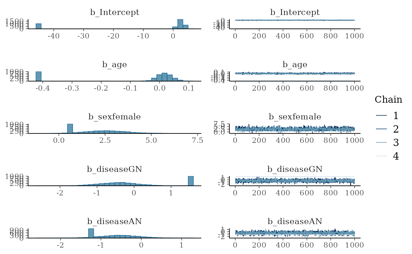
summary(fit3)
#> Warning: Inference for the model posterior has not converged (some Rhats are > 1.05). Be careful when analysing the results! We recommend running more iterations or setting stronger priors.
#> Family: lognormal
#> Links: mu = identity
#> Formula: time | cens(censored) ~ age * sex + disease + (1 | patient)
#> Data: kidney (Number of observations: 76)
#> Draws: 4 chains, each with iter = 2000; warmup = 1000; thin = 1;
#> total post-warmup draws = 4000
#>
#> Multilevel Hyperparameters:
#> ~patient (Number of levels: 38)
#> Estimate Est.Error l-95% CI u-95% CI Rhat Bulk_ESS Tail_ESS
#> sd(Intercept) 0.45 0.22 0.04 0.90 1.54 345 1387
#>
#> Regression Coefficients:
#> Estimate Est.Error l-95% CI u-95% CI Rhat Bulk_ESS Tail_ESS
#> Intercept -9.31 20.67 -45.08 4.36 1.58 7 12
#> age -0.09 0.19 -0.41 0.06 1.55 7 20
#> sexfemale 2.07 1.35 0.49 4.84 1.36 9 113
#> diseaseGN 0.06 0.96 -1.38 1.53 1.54 7 11
#> diseaseAN -0.71 0.52 -1.47 0.36 1.21 14 1434
#> diseasePKD 0.27 0.80 -0.67 1.83 1.31 10 167
#> age:sexfemale 0.48 0.88 -0.07 2.00 1.59 7 11
#>
#> Further Distributional Parameters:
#> Estimate Est.Error l-95% CI u-95% CI Rhat Bulk_ESS Tail_ESS
#> sigma 1.35 0.35 0.93 1.93 1.59 7 17
#>
#> Draws were sampled using sampling(NUTS). For each parameter, Bulk_ESS
#> and Tail_ESS are effective sample size measures, and Rhat is the potential
#> scale reduction factor on split chains (at convergence, Rhat = 1).
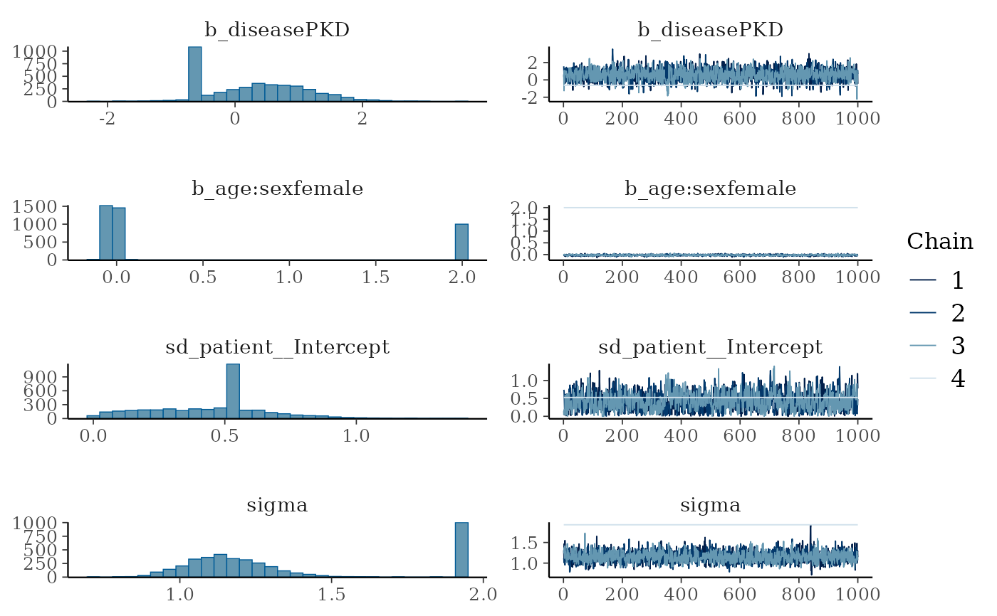
plot(fit3, ask = FALSE)
WAIC(fit2)
#> Warning:
#> 4 (0.7%) p_waic estimates greater than 0.4. We recommend trying loo instead.
#>
#> Computed from 2000 by 572 log-likelihood matrix.
#>
#> Estimate SE
#> elpd_waic -459.6 17.5
#> p_waic 8.3 1.2
#> waic 919.2 35.1
#>
#> 4 (0.7%) p_waic estimates greater than 0.4. We recommend trying loo instead.
# Survival regression modeling the time between the first
# and second recurrence of an infection in kidney patients.
fit3 <- brm(time | cens(censored) ~ age * sex + disease + (1|patient),
data = kidney, family = lognormal())
#> Compiling Stan program...
#> Start sampling
#>
#> SAMPLING FOR MODEL 'anon_model' NOW (CHAIN 1).
#> Chain 1: Rejecting initial value:
#> Chain 1: Log probability evaluates to log(0), i.e. negative infinity.
#> Chain 1: Stan can't start sampling from this initial value.
#> Chain 1:
#> Chain 1: Gradient evaluation took 2.6e-05 seconds
#> Chain 1: 1000 transitions using 10 leapfrog steps per transition would take 0.26 seconds.
#> Chain 1: Adjust your expectations accordingly!
#> Chain 1:
#> Chain 1:
#> Chain 1: Iteration: 1 / 2000 [ 0%] (Warmup)
#> Chain 1: Iteration: 200 / 2000 [ 10%] (Warmup)
#> Chain 1: Iteration: 400 / 2000 [ 20%] (Warmup)
#> Chain 1: Iteration: 600 / 2000 [ 30%] (Warmup)
#> Chain 1: Iteration: 800 / 2000 [ 40%] (Warmup)
#> Chain 1: Iteration: 1000 / 2000 [ 50%] (Warmup)
#> Chain 1: Iteration: 1001 / 2000 [ 50%] (Sampling)
#> Chain 1: Iteration: 1200 / 2000 [ 60%] (Sampling)
#> Chain 1: Iteration: 1400 / 2000 [ 70%] (Sampling)
#> Chain 1: Iteration: 1600 / 2000 [ 80%] (Sampling)
#> Chain 1: Iteration: 1800 / 2000 [ 90%] (Sampling)
#> Chain 1: Iteration: 2000 / 2000 [100%] (Sampling)
#> Chain 1:
#> Chain 1: Elapsed Time: 1.008 seconds (Warm-up)
#> Chain 1: 0.395 seconds (Sampling)
#> Chain 1: 1.403 seconds (Total)
#> Chain 1:
#>
#> SAMPLING FOR MODEL 'anon_model' NOW (CHAIN 2).
#> Chain 2: Rejecting initial value:
#> Chain 2: Log probability evaluates to log(0), i.e. negative infinity.
#> Chain 2: Stan can't start sampling from this initial value.
#> Chain 2:
#> Chain 2: Gradient evaluation took 1.7e-05 seconds
#> Chain 2: 1000 transitions using 10 leapfrog steps per transition would take 0.17 seconds.
#> Chain 2: Adjust your expectations accordingly!
#> Chain 2:
#> Chain 2:
#> Chain 2: Iteration: 1 / 2000 [ 0%] (Warmup)
#> Chain 2: Iteration: 200 / 2000 [ 10%] (Warmup)
#> Chain 2: Iteration: 400 / 2000 [ 20%] (Warmup)
#> Chain 2: Iteration: 600 / 2000 [ 30%] (Warmup)
#> Chain 2: Iteration: 800 / 2000 [ 40%] (Warmup)
#> Chain 2: Iteration: 1000 / 2000 [ 50%] (Warmup)
#> Chain 2: Iteration: 1001 / 2000 [ 50%] (Sampling)
#> Chain 2: Iteration: 1200 / 2000 [ 60%] (Sampling)
#> Chain 2: Iteration: 1400 / 2000 [ 70%] (Sampling)
#> Chain 2: Iteration: 1600 / 2000 [ 80%] (Sampling)
#> Chain 2: Iteration: 1800 / 2000 [ 90%] (Sampling)
#> Chain 2: Iteration: 2000 / 2000 [100%] (Sampling)
#> Chain 2:
#> Chain 2: Elapsed Time: 1.112 seconds (Warm-up)
#> Chain 2: 0.389 seconds (Sampling)
#> Chain 2: 1.501 seconds (Total)
#> Chain 2:
#>
#> SAMPLING FOR MODEL 'anon_model' NOW (CHAIN 3).
#> Chain 3: Rejecting initial value:
#> Chain 3: Log probability evaluates to log(0), i.e. negative infinity.
#> Chain 3: Stan can't start sampling from this initial value.
#> Chain 3:
#> Chain 3: Gradient evaluation took 1.7e-05 seconds
#> Chain 3: 1000 transitions using 10 leapfrog steps per transition would take 0.17 seconds.
#> Chain 3: Adjust your expectations accordingly!
#> Chain 3:
#> Chain 3:
#> Chain 3: Iteration: 1 / 2000 [ 0%] (Warmup)
#> Chain 3: Iteration: 200 / 2000 [ 10%] (Warmup)
#> Chain 3: Iteration: 400 / 2000 [ 20%] (Warmup)
#> Chain 3: Iteration: 600 / 2000 [ 30%] (Warmup)
#> Chain 3: Iteration: 800 / 2000 [ 40%] (Warmup)
#> Chain 3: Iteration: 1000 / 2000 [ 50%] (Warmup)
#> Chain 3: Iteration: 1001 / 2000 [ 50%] (Sampling)
#> Chain 3: Iteration: 1200 / 2000 [ 60%] (Sampling)
#> Chain 3: Iteration: 1400 / 2000 [ 70%] (Sampling)
#> Chain 3: Iteration: 1600 / 2000 [ 80%] (Sampling)
#> Chain 3: Iteration: 1800 / 2000 [ 90%] (Sampling)
#> Chain 3: Iteration: 2000 / 2000 [100%] (Sampling)
#> Chain 3:
#> Chain 3: Elapsed Time: 1.008 seconds (Warm-up)
#> Chain 3: 0.362 seconds (Sampling)
#> Chain 3: 1.37 seconds (Total)
#> Chain 3:
#>
#> SAMPLING FOR MODEL 'anon_model' NOW (CHAIN 4).
#> Chain 4: Rejecting initial value:
#> Chain 4: Log probability evaluates to log(0), i.e. negative infinity.
#> Chain 4: Stan can't start sampling from this initial value.
#> Chain 4:
#> Chain 4: Gradient evaluation took 1.6e-05 seconds
#> Chain 4: 1000 transitions using 10 leapfrog steps per transition would take 0.16 seconds.
#> Chain 4: Adjust your expectations accordingly!
#> Chain 4:
#> Chain 4:
#> Chain 4: Iteration: 1 / 2000 [ 0%] (Warmup)
#> Chain 4: Iteration: 200 / 2000 [ 10%] (Warmup)
#> Chain 4: Iteration: 400 / 2000 [ 20%] (Warmup)
#> Chain 4: Iteration: 600 / 2000 [ 30%] (Warmup)
#> Chain 4: Iteration: 800 / 2000 [ 40%] (Warmup)
#> Chain 4: Iteration: 1000 / 2000 [ 50%] (Warmup)
#> Chain 4: Iteration: 1001 / 2000 [ 50%] (Sampling)
#> Chain 4: Iteration: 1200 / 2000 [ 60%] (Sampling)
#> Chain 4: Iteration: 1400 / 2000 [ 70%] (Sampling)
#> Chain 4: Iteration: 1600 / 2000 [ 80%] (Sampling)
#> Chain 4: Iteration: 1800 / 2000 [ 90%] (Sampling)
#> Chain 4: Iteration: 2000 / 2000 [100%] (Sampling)
#> Chain 4:
#> Chain 4: Elapsed Time: 12.339 seconds (Warm-up)
#> Chain 4: 12.637 seconds (Sampling)
#> Chain 4: 24.976 seconds (Total)
#> Chain 4:
#> Warning: There were 1000 transitions after warmup that exceeded the maximum treedepth. Increase max_treedepth above 10. See
#> https://mc-stan.org/misc/warnings.html#maximum-treedepth-exceeded
#> Warning: Examine the pairs() plot to diagnose sampling problems
#> Warning: The largest R-hat is 1.59, indicating chains have not mixed.
#> Running the chains for more iterations may help. See
#> https://mc-stan.org/misc/warnings.html#r-hat
#> Warning: Bulk Effective Samples Size (ESS) is too low, indicating posterior means and medians may be unreliable.
#> Running the chains for more iterations may help. See
#> https://mc-stan.org/misc/warnings.html#bulk-ess
#> Warning: Tail Effective Samples Size (ESS) is too low, indicating posterior variances and tail quantiles may be unreliable.
#> Running the chains for more iterations may help. See
#> https://mc-stan.org/misc/warnings.html#tail-ess
summary(fit3)
#> Warning: Inference for the model posterior has not converged (some Rhats are > 1.05). Be careful when analysing the results! We recommend running more iterations or setting stronger priors.
#> Family: lognormal
#> Links: mu = identity
#> Formula: time | cens(censored) ~ age * sex + disease + (1 | patient)
#> Data: kidney (Number of observations: 76)
#> Draws: 4 chains, each with iter = 2000; warmup = 1000; thin = 1;
#> total post-warmup draws = 4000
#>
#> Multilevel Hyperparameters:
#> ~patient (Number of levels: 38)
#> Estimate Est.Error l-95% CI u-95% CI Rhat Bulk_ESS Tail_ESS
#> sd(Intercept) 0.45 0.22 0.04 0.90 1.54 345 1387
#>
#> Regression Coefficients:
#> Estimate Est.Error l-95% CI u-95% CI Rhat Bulk_ESS Tail_ESS
#> Intercept -9.31 20.67 -45.08 4.36 1.58 7 12
#> age -0.09 0.19 -0.41 0.06 1.55 7 20
#> sexfemale 2.07 1.35 0.49 4.84 1.36 9 113
#> diseaseGN 0.06 0.96 -1.38 1.53 1.54 7 11
#> diseaseAN -0.71 0.52 -1.47 0.36 1.21 14 1434
#> diseasePKD 0.27 0.80 -0.67 1.83 1.31 10 167
#> age:sexfemale 0.48 0.88 -0.07 2.00 1.59 7 11
#>
#> Further Distributional Parameters:
#> Estimate Est.Error l-95% CI u-95% CI Rhat Bulk_ESS Tail_ESS
#> sigma 1.35 0.35 0.93 1.93 1.59 7 17
#>
#> Draws were sampled using sampling(NUTS). For each parameter, Bulk_ESS
#> and Tail_ESS are effective sample size measures, and Rhat is the potential
#> scale reduction factor on split chains (at convergence, Rhat = 1).
plot(fit3, ask = FALSE)
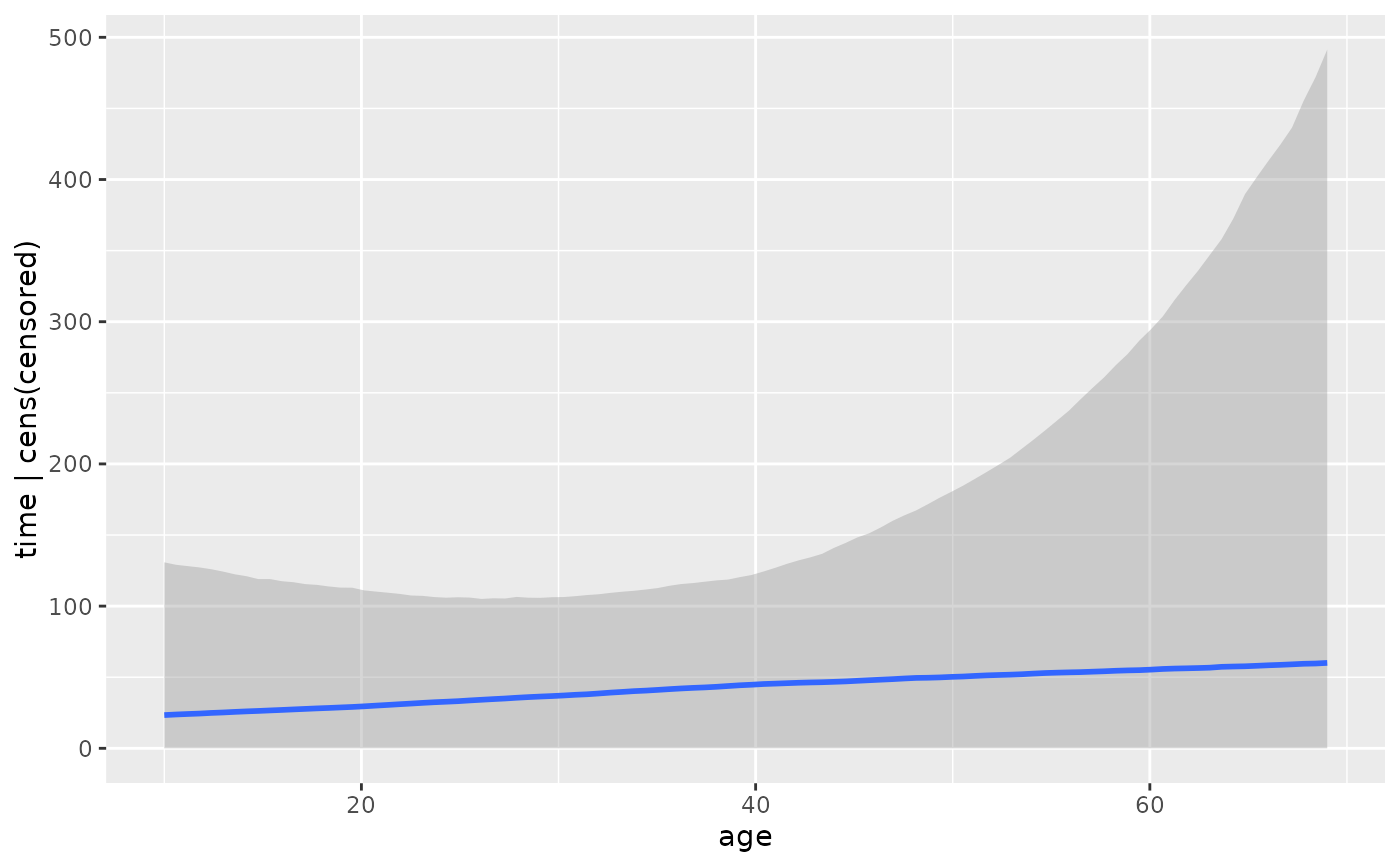
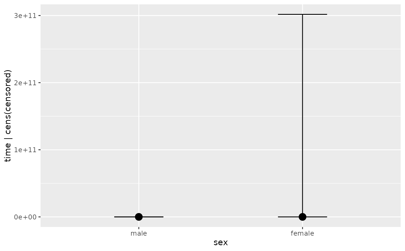
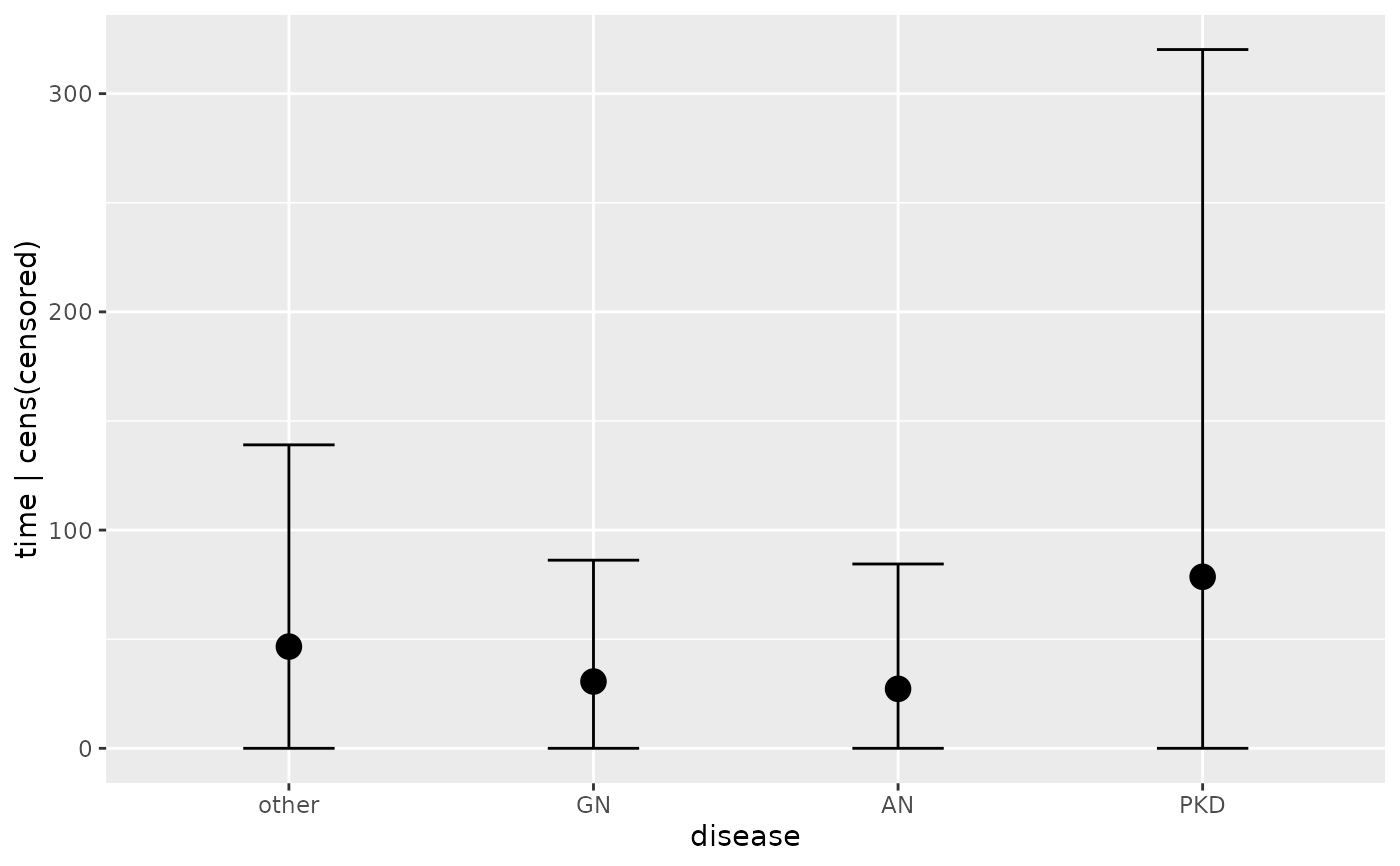
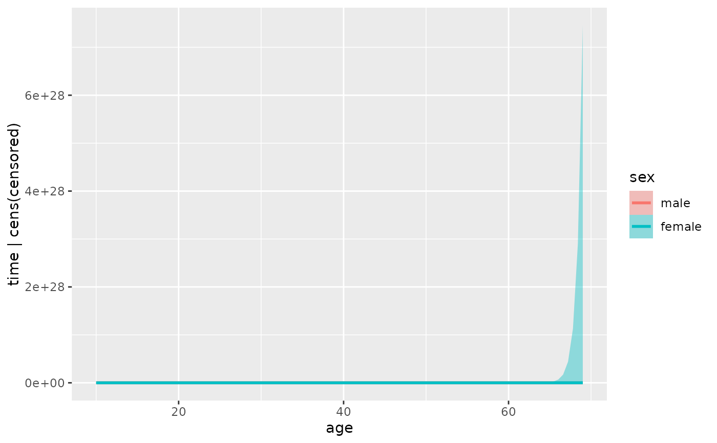
 plot(conditional_effects(fit3), ask = FALSE)
 # Probit regression using the binomial family
ntrials <- sample(1:10, 100, TRUE)
success <- rbinom(100, size = ntrials, prob = 0.4)
x <- rnorm(100)
data4 <- data.frame(ntrials, success, x)
fit4 <- brm(success | trials(ntrials) ~ x, data = data4,
family = binomial("probit"))
#> Compiling Stan program...
#> Start sampling
#>
#> SAMPLING FOR MODEL 'anon_model' NOW (CHAIN 1).
#> Chain 1:
#> Chain 1: Gradient evaluation took 2.3e-05 seconds
#> Chain 1: 1000 transitions using 10 leapfrog steps per transition would take 0.23 seconds.
#> Chain 1: Adjust your expectations accordingly!
#> Chain 1:
#> Chain 1:
#> Chain 1: Iteration: 1 / 2000 [ 0%] (Warmup)
#> Chain 1: Iteration: 200 / 2000 [ 10%] (Warmup)
#> Chain 1: Iteration: 400 / 2000 [ 20%] (Warmup)
#> Chain 1: Iteration: 600 / 2000 [ 30%] (Warmup)
#> Chain 1: Iteration: 800 / 2000 [ 40%] (Warmup)
#> Chain 1: Iteration: 1000 / 2000 [ 50%] (Warmup)
#> Chain 1: Iteration: 1001 / 2000 [ 50%] (Sampling)
#> Chain 1: Iteration: 1200 / 2000 [ 60%] (Sampling)
#> Chain 1: Iteration: 1400 / 2000 [ 70%] (Sampling)
#> Chain 1: Iteration: 1600 / 2000 [ 80%] (Sampling)
#> Chain 1: Iteration: 1800 / 2000 [ 90%] (Sampling)
#> Chain 1: Iteration: 2000 / 2000 [100%] (Sampling)
#> Chain 1:
#> Chain 1: Elapsed Time: 0.072 seconds (Warm-up)
#> Chain 1: 0.071 seconds (Sampling)
#> Chain 1: 0.143 seconds (Total)
#> Chain 1:
#>
#> SAMPLING FOR MODEL 'anon_model' NOW (CHAIN 2).
#> Chain 2:
#> Chain 2: Gradient evaluation took 1.9e-05 seconds
#> Chain 2: 1000 transitions using 10 leapfrog steps per transition would take 0.19 seconds.
#> Chain 2: Adjust your expectations accordingly!
#> Chain 2:
#> Chain 2:
#> Chain 2: Iteration: 1 / 2000 [ 0%] (Warmup)
#> Chain 2: Iteration: 200 / 2000 [ 10%] (Warmup)
#> Chain 2: Iteration: 400 / 2000 [ 20%] (Warmup)
#> Chain 2: Iteration: 600 / 2000 [ 30%] (Warmup)
#> Chain 2: Iteration: 800 / 2000 [ 40%] (Warmup)
#> Chain 2: Iteration: 1000 / 2000 [ 50%] (Warmup)
#> Chain 2: Iteration: 1001 / 2000 [ 50%] (Sampling)
#> Chain 2: Iteration: 1200 / 2000 [ 60%] (Sampling)
#> Chain 2: Iteration: 1400 / 2000 [ 70%] (Sampling)
#> Chain 2: Iteration: 1600 / 2000 [ 80%] (Sampling)
#> Chain 2: Iteration: 1800 / 2000 [ 90%] (Sampling)
#> Chain 2: Iteration: 2000 / 2000 [100%] (Sampling)
#> Chain 2:
#> Chain 2: Elapsed Time: 0.074 seconds (Warm-up)
#> Chain 2: 0.078 seconds (Sampling)
#> Chain 2: 0.152 seconds (Total)
#> Chain 2:
#>
#> SAMPLING FOR MODEL 'anon_model' NOW (CHAIN 3).
#> Chain 3:
#> Chain 3: Gradient evaluation took 1.8e-05 seconds
#> Chain 3: 1000 transitions using 10 leapfrog steps per transition would take 0.18 seconds.
#> Chain 3: Adjust your expectations accordingly!
#> Chain 3:
#> Chain 3:
#> Chain 3: Iteration: 1 / 2000 [ 0%] (Warmup)
#> Chain 3: Iteration: 200 / 2000 [ 10%] (Warmup)
#> Chain 3: Iteration: 400 / 2000 [ 20%] (Warmup)
#> Chain 3: Iteration: 600 / 2000 [ 30%] (Warmup)
#> Chain 3: Iteration: 800 / 2000 [ 40%] (Warmup)
#> Chain 3: Iteration: 1000 / 2000 [ 50%] (Warmup)
#> Chain 3: Iteration: 1001 / 2000 [ 50%] (Sampling)
#> Chain 3: Iteration: 1200 / 2000 [ 60%] (Sampling)
#> Chain 3: Iteration: 1400 / 2000 [ 70%] (Sampling)
#> Chain 3: Iteration: 1600 / 2000 [ 80%] (Sampling)
#> Chain 3: Iteration: 1800 / 2000 [ 90%] (Sampling)
#> Chain 3: Iteration: 2000 / 2000 [100%] (Sampling)
#> Chain 3:
#> Chain 3: Elapsed Time: 0.072 seconds (Warm-up)
#> Chain 3: 0.074 seconds (Sampling)
#> Chain 3: 0.146 seconds (Total)
#> Chain 3:
#>
#> SAMPLING FOR MODEL 'anon_model' NOW (CHAIN 4).
#> Chain 4:
#> Chain 4: Gradient evaluation took 1.7e-05 seconds
#> Chain 4: 1000 transitions using 10 leapfrog steps per transition would take 0.17 seconds.
#> Chain 4: Adjust your expectations accordingly!
#> Chain 4:
#> Chain 4:
#> Chain 4: Iteration: 1 / 2000 [ 0%] (Warmup)
#> Chain 4: Iteration: 200 / 2000 [ 10%] (Warmup)
#> Chain 4: Iteration: 400 / 2000 [ 20%] (Warmup)
#> Chain 4: Iteration: 600 / 2000 [ 30%] (Warmup)
#> Chain 4: Iteration: 800 / 2000 [ 40%] (Warmup)
#> Chain 4: Iteration: 1000 / 2000 [ 50%] (Warmup)
#> Chain 4: Iteration: 1001 / 2000 [ 50%] (Sampling)
#> Chain 4: Iteration: 1200 / 2000 [ 60%] (Sampling)
#> Chain 4: Iteration: 1400 / 2000 [ 70%] (Sampling)
#> Chain 4: Iteration: 1600 / 2000 [ 80%] (Sampling)
#> Chain 4: Iteration: 1800 / 2000 [ 90%] (Sampling)
#> Chain 4: Iteration: 2000 / 2000 [100%] (Sampling)
#> Chain 4:
#> Chain 4: Elapsed Time: 0.072 seconds (Warm-up)
#> Chain 4: 0.064 seconds (Sampling)
#> Chain 4: 0.136 seconds (Total)
#> Chain 4:
summary(fit4)
#> Family: binomial
#> Links: mu = probit
#> Formula: success | trials(ntrials) ~ x
#> Data: data4 (Number of observations: 100)
#> Draws: 4 chains, each with iter = 2000; warmup = 1000; thin = 1;
#> total post-warmup draws = 4000
#>
#> Regression Coefficients:
#> Estimate Est.Error l-95% CI u-95% CI Rhat Bulk_ESS Tail_ESS
#> Intercept -0.22 0.06 -0.33 -0.11 1.00 3413 2925
#> x -0.01 0.05 -0.12 0.09 1.00 3676 2881
#>
#> Draws were sampled using sampling(NUTS). For each parameter, Bulk_ESS
#> and Tail_ESS are effective sample size measures, and Rhat is the potential
#> scale reduction factor on split chains (at convergence, Rhat = 1).
# Non-linear Gaussian model
fit5 <- brm(
bf(cum ~ ult * (1 - exp(-(dev/theta)^omega)),
ult ~ 1 + (1|AY), omega ~ 1, theta ~ 1,
nl = TRUE),
data = loss, family = gaussian(),
prior = c(
prior(normal(5000, 1000), nlpar = "ult"),
prior(normal(1, 2), nlpar = "omega"),
prior(normal(45, 10), nlpar = "theta")
),
control = list(adapt_delta = 0.9)
)
#> Compiling Stan program...
#> Start sampling
#>
#> SAMPLING FOR MODEL 'anon_model' NOW (CHAIN 1).
#> Chain 1: Rejecting initial value:
#> Chain 1: Error evaluating the log probability at the initial value.
#> Chain 1: Exception: normal_lpdf: Location parameter[1] is nan, but must be finite! (in 'anon_model', line 68, column 4 to column 41)
#> Chain 1: Rejecting initial value:
#> Chain 1: Error evaluating the log probability at the initial value.
#> Chain 1: Exception: normal_lpdf: Location parameter[1] is nan, but must be finite! (in 'anon_model', line 68, column 4 to column 41)
#> Chain 1:
#> Chain 1: Gradient evaluation took 3e-05 seconds
#> Chain 1: 1000 transitions using 10 leapfrog steps per transition would take 0.3 seconds.
#> Chain 1: Adjust your expectations accordingly!
#> Chain 1:
#> Chain 1:
#> Chain 1: Iteration: 1 / 2000 [ 0%] (Warmup)
#> Chain 1: Iteration: 200 / 2000 [ 10%] (Warmup)
#> Chain 1: Iteration: 400 / 2000 [ 20%] (Warmup)
#> Chain 1: Iteration: 600 / 2000 [ 30%] (Warmup)
#> Chain 1: Iteration: 800 / 2000 [ 40%] (Warmup)
#> Chain 1: Iteration: 1000 / 2000 [ 50%] (Warmup)
#> Chain 1: Iteration: 1001 / 2000 [ 50%] (Sampling)
#> Chain 1: Iteration: 1200 / 2000 [ 60%] (Sampling)
#> Chain 1: Iteration: 1400 / 2000 [ 70%] (Sampling)
#> Chain 1: Iteration: 1600 / 2000 [ 80%] (Sampling)
#> Chain 1: Iteration: 1800 / 2000 [ 90%] (Sampling)
#> Chain 1: Iteration: 2000 / 2000 [100%] (Sampling)
#> Chain 1:
#> Chain 1: Elapsed Time: 2.058 seconds (Warm-up)
#> Chain 1: 1.192 seconds (Sampling)
#> Chain 1: 3.25 seconds (Total)
#> Chain 1:
#>
#> SAMPLING FOR MODEL 'anon_model' NOW (CHAIN 2).
#> Chain 2: Rejecting initial value:
#> Chain 2: Error evaluating the log probability at the initial value.
#> Chain 2: Exception: normal_lpdf: Location parameter[1] is nan, but must be finite! (in 'anon_model', line 68, column 4 to column 41)
#> Chain 2: Rejecting initial value:
#> Chain 2: Error evaluating the log probability at the initial value.
#> Chain 2: Exception: normal_lpdf: Location parameter[1] is nan, but must be finite! (in 'anon_model', line 68, column 4 to column 41)
#> Chain 2: Rejecting initial value:
#> Chain 2: Error evaluating the log probability at the initial value.
#> Chain 2: Exception: normal_lpdf: Location parameter[1] is nan, but must be finite! (in 'anon_model', line 68, column 4 to column 41)
#> Chain 2: Rejecting initial value:
#> Chain 2: Error evaluating the log probability at the initial value.
#> Chain 2: Exception: normal_lpdf: Location parameter[1] is nan, but must be finite! (in 'anon_model', line 68, column 4 to column 41)
#> Chain 2: Rejecting initial value:
#> Chain 2: Error evaluating the log probability at the initial value.
#> Chain 2: Exception: normal_lpdf: Location parameter[1] is nan, but must be finite! (in 'anon_model', line 68, column 4 to column 41)
#> Chain 2:
#> Chain 2: Gradient evaluation took 2.2e-05 seconds
#> Chain 2: 1000 transitions using 10 leapfrog steps per transition would take 0.22 seconds.
#> Chain 2: Adjust your expectations accordingly!
#> Chain 2:
#> Chain 2:
#> Chain 2: Iteration: 1 / 2000 [ 0%] (Warmup)
#> Chain 2: Iteration: 200 / 2000 [ 10%] (Warmup)
#> Chain 2: Iteration: 400 / 2000 [ 20%] (Warmup)
#> Chain 2: Iteration: 600 / 2000 [ 30%] (Warmup)
#> Chain 2: Iteration: 800 / 2000 [ 40%] (Warmup)
#> Chain 2: Iteration: 1000 / 2000 [ 50%] (Warmup)
#> Chain 2: Iteration: 1001 / 2000 [ 50%] (Sampling)
#> Chain 2: Iteration: 1200 / 2000 [ 60%] (Sampling)
#> Chain 2: Iteration: 1400 / 2000 [ 70%] (Sampling)
#> Chain 2: Iteration: 1600 / 2000 [ 80%] (Sampling)
#> Chain 2: Iteration: 1800 / 2000 [ 90%] (Sampling)
#> Chain 2: Iteration: 2000 / 2000 [100%] (Sampling)
#> Chain 2:
#> Chain 2: Elapsed Time: 2.394 seconds (Warm-up)
#> Chain 2: 1.232 seconds (Sampling)
#> Chain 2: 3.626 seconds (Total)
#> Chain 2:
#>
#> SAMPLING FOR MODEL 'anon_model' NOW (CHAIN 3).
#> Chain 3: Rejecting initial value:
#> Chain 3: Error evaluating the log probability at the initial value.
#> Chain 3: Exception: normal_lpdf: Location parameter[1] is nan, but must be finite! (in 'anon_model', line 68, column 4 to column 41)
#> Chain 3:
#> Chain 3: Gradient evaluation took 2.6e-05 seconds
#> Chain 3: 1000 transitions using 10 leapfrog steps per transition would take 0.26 seconds.
#> Chain 3: Adjust your expectations accordingly!
#> Chain 3:
#> Chain 3:
#> Chain 3: Iteration: 1 / 2000 [ 0%] (Warmup)
#> Chain 3: Iteration: 200 / 2000 [ 10%] (Warmup)
#> Chain 3: Iteration: 400 / 2000 [ 20%] (Warmup)
#> Chain 3: Iteration: 600 / 2000 [ 30%] (Warmup)
#> Chain 3: Iteration: 800 / 2000 [ 40%] (Warmup)
#> Chain 3: Iteration: 1000 / 2000 [ 50%] (Warmup)
#> Chain 3: Iteration: 1001 / 2000 [ 50%] (Sampling)
#> Chain 3: Iteration: 1200 / 2000 [ 60%] (Sampling)
#> Chain 3: Iteration: 1400 / 2000 [ 70%] (Sampling)
#> Chain 3: Iteration: 1600 / 2000 [ 80%] (Sampling)
#> Chain 3: Iteration: 1800 / 2000 [ 90%] (Sampling)
#> Chain 3: Iteration: 2000 / 2000 [100%] (Sampling)
#> Chain 3:
#> Chain 3: Elapsed Time: 2.388 seconds (Warm-up)
#> Chain 3: 1.27 seconds (Sampling)
#> Chain 3: 3.658 seconds (Total)
#> Chain 3:
#>
#> SAMPLING FOR MODEL 'anon_model' NOW (CHAIN 4).
#> Chain 4: Rejecting initial value:
#> Chain 4: Error evaluating the log probability at the initial value.
#> Chain 4: Exception: normal_lpdf: Location parameter[1] is nan, but must be finite! (in 'anon_model', line 68, column 4 to column 41)
#> Chain 4: Rejecting initial value:
#> Chain 4: Error evaluating the log probability at the initial value.
#> Chain 4: Exception: normal_lpdf: Location parameter[1] is nan, but must be finite! (in 'anon_model', line 68, column 4 to column 41)
#> Chain 4: Rejecting initial value:
#> Chain 4: Error evaluating the log probability at the initial value.
#> Chain 4: Exception: normal_lpdf: Location parameter[1] is nan, but must be finite! (in 'anon_model', line 68, column 4 to column 41)
#> Chain 4:
#> Chain 4: Gradient evaluation took 2.2e-05 seconds
#> Chain 4: 1000 transitions using 10 leapfrog steps per transition would take 0.22 seconds.
#> Chain 4: Adjust your expectations accordingly!
#> Chain 4:
#> Chain 4:
#> Chain 4: Iteration: 1 / 2000 [ 0%] (Warmup)
#> Chain 4: Iteration: 200 / 2000 [ 10%] (Warmup)
#> Chain 4: Iteration: 400 / 2000 [ 20%] (Warmup)
#> Chain 4: Iteration: 600 / 2000 [ 30%] (Warmup)
#> Chain 4: Iteration: 800 / 2000 [ 40%] (Warmup)
#> Chain 4: Iteration: 1000 / 2000 [ 50%] (Warmup)
#> Chain 4: Iteration: 1001 / 2000 [ 50%] (Sampling)
#> Chain 4: Iteration: 1200 / 2000 [ 60%] (Sampling)
#> Chain 4: Iteration: 1400 / 2000 [ 70%] (Sampling)
#> Chain 4: Iteration: 1600 / 2000 [ 80%] (Sampling)
#> Chain 4: Iteration: 1800 / 2000 [ 90%] (Sampling)
#> Chain 4: Iteration: 2000 / 2000 [100%] (Sampling)
#> Chain 4:
#> Chain 4: Elapsed Time: 2.349 seconds (Warm-up)
#> Chain 4: 1.111 seconds (Sampling)
#> Chain 4: 3.46 seconds (Total)
#> Chain 4:
summary(fit5)
#> Family: gaussian
#> Links: mu = identity
#> Formula: cum ~ ult * (1 - exp(-(dev/theta)^omega))
#> ult ~ 1 + (1 | AY)
#> omega ~ 1
#> theta ~ 1
#> Data: loss (Number of observations: 55)
#> Draws: 4 chains, each with iter = 2000; warmup = 1000; thin = 1;
#> total post-warmup draws = 4000
#>
#> Multilevel Hyperparameters:
#> ~AY (Number of levels: 10)
#> Estimate Est.Error l-95% CI u-95% CI Rhat Bulk_ESS Tail_ESS
#> sd(ult_Intercept) 751.87 237.81 427.80 1332.92 1.00 1286 1743
#>
#> Regression Coefficients:
#> Estimate Est.Error l-95% CI u-95% CI Rhat Bulk_ESS Tail_ESS
#> ult_Intercept 5295.83 299.78 4725.94 5916.82 1.01 934 1567
#> omega_Intercept 1.34 0.05 1.24 1.44 1.00 2455 2372
#> theta_Intercept 46.18 2.16 42.40 50.81 1.00 2191 2052
#>
#> Further Distributional Parameters:
#> Estimate Est.Error l-95% CI u-95% CI Rhat Bulk_ESS Tail_ESS
#> sigma 139.77 15.20 114.20 172.91 1.00 3063 2671
#>
#> Draws were sampled using sampling(NUTS). For each parameter, Bulk_ESS
#> and Tail_ESS are effective sample size measures, and Rhat is the potential
#> scale reduction factor on split chains (at convergence, Rhat = 1).
conditional_effects(fit5)
# Probit regression using the binomial family
ntrials <- sample(1:10, 100, TRUE)
success <- rbinom(100, size = ntrials, prob = 0.4)
x <- rnorm(100)
data4 <- data.frame(ntrials, success, x)
fit4 <- brm(success | trials(ntrials) ~ x, data = data4,
family = binomial("probit"))
#> Compiling Stan program...
#> Start sampling
#>
#> SAMPLING FOR MODEL 'anon_model' NOW (CHAIN 1).
#> Chain 1:
#> Chain 1: Gradient evaluation took 2.3e-05 seconds
#> Chain 1: 1000 transitions using 10 leapfrog steps per transition would take 0.23 seconds.
#> Chain 1: Adjust your expectations accordingly!
#> Chain 1:
#> Chain 1:
#> Chain 1: Iteration: 1 / 2000 [ 0%] (Warmup)
#> Chain 1: Iteration: 200 / 2000 [ 10%] (Warmup)
#> Chain 1: Iteration: 400 / 2000 [ 20%] (Warmup)
#> Chain 1: Iteration: 600 / 2000 [ 30%] (Warmup)
#> Chain 1: Iteration: 800 / 2000 [ 40%] (Warmup)
#> Chain 1: Iteration: 1000 / 2000 [ 50%] (Warmup)
#> Chain 1: Iteration: 1001 / 2000 [ 50%] (Sampling)
#> Chain 1: Iteration: 1200 / 2000 [ 60%] (Sampling)
#> Chain 1: Iteration: 1400 / 2000 [ 70%] (Sampling)
#> Chain 1: Iteration: 1600 / 2000 [ 80%] (Sampling)
#> Chain 1: Iteration: 1800 / 2000 [ 90%] (Sampling)
#> Chain 1: Iteration: 2000 / 2000 [100%] (Sampling)
#> Chain 1:
#> Chain 1: Elapsed Time: 0.072 seconds (Warm-up)
#> Chain 1: 0.071 seconds (Sampling)
#> Chain 1: 0.143 seconds (Total)
#> Chain 1:
#>
#> SAMPLING FOR MODEL 'anon_model' NOW (CHAIN 2).
#> Chain 2:
#> Chain 2: Gradient evaluation took 1.9e-05 seconds
#> Chain 2: 1000 transitions using 10 leapfrog steps per transition would take 0.19 seconds.
#> Chain 2: Adjust your expectations accordingly!
#> Chain 2:
#> Chain 2:
#> Chain 2: Iteration: 1 / 2000 [ 0%] (Warmup)
#> Chain 2: Iteration: 200 / 2000 [ 10%] (Warmup)
#> Chain 2: Iteration: 400 / 2000 [ 20%] (Warmup)
#> Chain 2: Iteration: 600 / 2000 [ 30%] (Warmup)
#> Chain 2: Iteration: 800 / 2000 [ 40%] (Warmup)
#> Chain 2: Iteration: 1000 / 2000 [ 50%] (Warmup)
#> Chain 2: Iteration: 1001 / 2000 [ 50%] (Sampling)
#> Chain 2: Iteration: 1200 / 2000 [ 60%] (Sampling)
#> Chain 2: Iteration: 1400 / 2000 [ 70%] (Sampling)
#> Chain 2: Iteration: 1600 / 2000 [ 80%] (Sampling)
#> Chain 2: Iteration: 1800 / 2000 [ 90%] (Sampling)
#> Chain 2: Iteration: 2000 / 2000 [100%] (Sampling)
#> Chain 2:
#> Chain 2: Elapsed Time: 0.074 seconds (Warm-up)
#> Chain 2: 0.078 seconds (Sampling)
#> Chain 2: 0.152 seconds (Total)
#> Chain 2:
#>
#> SAMPLING FOR MODEL 'anon_model' NOW (CHAIN 3).
#> Chain 3:
#> Chain 3: Gradient evaluation took 1.8e-05 seconds
#> Chain 3: 1000 transitions using 10 leapfrog steps per transition would take 0.18 seconds.
#> Chain 3: Adjust your expectations accordingly!
#> Chain 3:
#> Chain 3:
#> Chain 3: Iteration: 1 / 2000 [ 0%] (Warmup)
#> Chain 3: Iteration: 200 / 2000 [ 10%] (Warmup)
#> Chain 3: Iteration: 400 / 2000 [ 20%] (Warmup)
#> Chain 3: Iteration: 600 / 2000 [ 30%] (Warmup)
#> Chain 3: Iteration: 800 / 2000 [ 40%] (Warmup)
#> Chain 3: Iteration: 1000 / 2000 [ 50%] (Warmup)
#> Chain 3: Iteration: 1001 / 2000 [ 50%] (Sampling)
#> Chain 3: Iteration: 1200 / 2000 [ 60%] (Sampling)
#> Chain 3: Iteration: 1400 / 2000 [ 70%] (Sampling)
#> Chain 3: Iteration: 1600 / 2000 [ 80%] (Sampling)
#> Chain 3: Iteration: 1800 / 2000 [ 90%] (Sampling)
#> Chain 3: Iteration: 2000 / 2000 [100%] (Sampling)
#> Chain 3:
#> Chain 3: Elapsed Time: 0.072 seconds (Warm-up)
#> Chain 3: 0.074 seconds (Sampling)
#> Chain 3: 0.146 seconds (Total)
#> Chain 3:
#>
#> SAMPLING FOR MODEL 'anon_model' NOW (CHAIN 4).
#> Chain 4:
#> Chain 4: Gradient evaluation took 1.7e-05 seconds
#> Chain 4: 1000 transitions using 10 leapfrog steps per transition would take 0.17 seconds.
#> Chain 4: Adjust your expectations accordingly!
#> Chain 4:
#> Chain 4:
#> Chain 4: Iteration: 1 / 2000 [ 0%] (Warmup)
#> Chain 4: Iteration: 200 / 2000 [ 10%] (Warmup)
#> Chain 4: Iteration: 400 / 2000 [ 20%] (Warmup)
#> Chain 4: Iteration: 600 / 2000 [ 30%] (Warmup)
#> Chain 4: Iteration: 800 / 2000 [ 40%] (Warmup)
#> Chain 4: Iteration: 1000 / 2000 [ 50%] (Warmup)
#> Chain 4: Iteration: 1001 / 2000 [ 50%] (Sampling)
#> Chain 4: Iteration: 1200 / 2000 [ 60%] (Sampling)
#> Chain 4: Iteration: 1400 / 2000 [ 70%] (Sampling)
#> Chain 4: Iteration: 1600 / 2000 [ 80%] (Sampling)
#> Chain 4: Iteration: 1800 / 2000 [ 90%] (Sampling)
#> Chain 4: Iteration: 2000 / 2000 [100%] (Sampling)
#> Chain 4:
#> Chain 4: Elapsed Time: 0.072 seconds (Warm-up)
#> Chain 4: 0.064 seconds (Sampling)
#> Chain 4: 0.136 seconds (Total)
#> Chain 4:
summary(fit4)
#> Family: binomial
#> Links: mu = probit
#> Formula: success | trials(ntrials) ~ x
#> Data: data4 (Number of observations: 100)
#> Draws: 4 chains, each with iter = 2000; warmup = 1000; thin = 1;
#> total post-warmup draws = 4000
#>
#> Regression Coefficients:
#> Estimate Est.Error l-95% CI u-95% CI Rhat Bulk_ESS Tail_ESS
#> Intercept -0.22 0.06 -0.33 -0.11 1.00 3413 2925
#> x -0.01 0.05 -0.12 0.09 1.00 3676 2881
#>
#> Draws were sampled using sampling(NUTS). For each parameter, Bulk_ESS
#> and Tail_ESS are effective sample size measures, and Rhat is the potential
#> scale reduction factor on split chains (at convergence, Rhat = 1).
# Non-linear Gaussian model
fit5 <- brm(
bf(cum ~ ult * (1 - exp(-(dev/theta)^omega)),
ult ~ 1 + (1|AY), omega ~ 1, theta ~ 1,
nl = TRUE),
data = loss, family = gaussian(),
prior = c(
prior(normal(5000, 1000), nlpar = "ult"),
prior(normal(1, 2), nlpar = "omega"),
prior(normal(45, 10), nlpar = "theta")
),
control = list(adapt_delta = 0.9)
)
#> Compiling Stan program...
#> Start sampling
#>
#> SAMPLING FOR MODEL 'anon_model' NOW (CHAIN 1).
#> Chain 1: Rejecting initial value:
#> Chain 1: Error evaluating the log probability at the initial value.
#> Chain 1: Exception: normal_lpdf: Location parameter[1] is nan, but must be finite! (in 'anon_model', line 68, column 4 to column 41)
#> Chain 1: Rejecting initial value:
#> Chain 1: Error evaluating the log probability at the initial value.
#> Chain 1: Exception: normal_lpdf: Location parameter[1] is nan, but must be finite! (in 'anon_model', line 68, column 4 to column 41)
#> Chain 1:
#> Chain 1: Gradient evaluation took 3e-05 seconds
#> Chain 1: 1000 transitions using 10 leapfrog steps per transition would take 0.3 seconds.
#> Chain 1: Adjust your expectations accordingly!
#> Chain 1:
#> Chain 1:
#> Chain 1: Iteration: 1 / 2000 [ 0%] (Warmup)
#> Chain 1: Iteration: 200 / 2000 [ 10%] (Warmup)
#> Chain 1: Iteration: 400 / 2000 [ 20%] (Warmup)
#> Chain 1: Iteration: 600 / 2000 [ 30%] (Warmup)
#> Chain 1: Iteration: 800 / 2000 [ 40%] (Warmup)
#> Chain 1: Iteration: 1000 / 2000 [ 50%] (Warmup)
#> Chain 1: Iteration: 1001 / 2000 [ 50%] (Sampling)
#> Chain 1: Iteration: 1200 / 2000 [ 60%] (Sampling)
#> Chain 1: Iteration: 1400 / 2000 [ 70%] (Sampling)
#> Chain 1: Iteration: 1600 / 2000 [ 80%] (Sampling)
#> Chain 1: Iteration: 1800 / 2000 [ 90%] (Sampling)
#> Chain 1: Iteration: 2000 / 2000 [100%] (Sampling)
#> Chain 1:
#> Chain 1: Elapsed Time: 2.058 seconds (Warm-up)
#> Chain 1: 1.192 seconds (Sampling)
#> Chain 1: 3.25 seconds (Total)
#> Chain 1:
#>
#> SAMPLING FOR MODEL 'anon_model' NOW (CHAIN 2).
#> Chain 2: Rejecting initial value:
#> Chain 2: Error evaluating the log probability at the initial value.
#> Chain 2: Exception: normal_lpdf: Location parameter[1] is nan, but must be finite! (in 'anon_model', line 68, column 4 to column 41)
#> Chain 2: Rejecting initial value:
#> Chain 2: Error evaluating the log probability at the initial value.
#> Chain 2: Exception: normal_lpdf: Location parameter[1] is nan, but must be finite! (in 'anon_model', line 68, column 4 to column 41)
#> Chain 2: Rejecting initial value:
#> Chain 2: Error evaluating the log probability at the initial value.
#> Chain 2: Exception: normal_lpdf: Location parameter[1] is nan, but must be finite! (in 'anon_model', line 68, column 4 to column 41)
#> Chain 2: Rejecting initial value:
#> Chain 2: Error evaluating the log probability at the initial value.
#> Chain 2: Exception: normal_lpdf: Location parameter[1] is nan, but must be finite! (in 'anon_model', line 68, column 4 to column 41)
#> Chain 2: Rejecting initial value:
#> Chain 2: Error evaluating the log probability at the initial value.
#> Chain 2: Exception: normal_lpdf: Location parameter[1] is nan, but must be finite! (in 'anon_model', line 68, column 4 to column 41)
#> Chain 2:
#> Chain 2: Gradient evaluation took 2.2e-05 seconds
#> Chain 2: 1000 transitions using 10 leapfrog steps per transition would take 0.22 seconds.
#> Chain 2: Adjust your expectations accordingly!
#> Chain 2:
#> Chain 2:
#> Chain 2: Iteration: 1 / 2000 [ 0%] (Warmup)
#> Chain 2: Iteration: 200 / 2000 [ 10%] (Warmup)
#> Chain 2: Iteration: 400 / 2000 [ 20%] (Warmup)
#> Chain 2: Iteration: 600 / 2000 [ 30%] (Warmup)
#> Chain 2: Iteration: 800 / 2000 [ 40%] (Warmup)
#> Chain 2: Iteration: 1000 / 2000 [ 50%] (Warmup)
#> Chain 2: Iteration: 1001 / 2000 [ 50%] (Sampling)
#> Chain 2: Iteration: 1200 / 2000 [ 60%] (Sampling)
#> Chain 2: Iteration: 1400 / 2000 [ 70%] (Sampling)
#> Chain 2: Iteration: 1600 / 2000 [ 80%] (Sampling)
#> Chain 2: Iteration: 1800 / 2000 [ 90%] (Sampling)
#> Chain 2: Iteration: 2000 / 2000 [100%] (Sampling)
#> Chain 2:
#> Chain 2: Elapsed Time: 2.394 seconds (Warm-up)
#> Chain 2: 1.232 seconds (Sampling)
#> Chain 2: 3.626 seconds (Total)
#> Chain 2:
#>
#> SAMPLING FOR MODEL 'anon_model' NOW (CHAIN 3).
#> Chain 3: Rejecting initial value:
#> Chain 3: Error evaluating the log probability at the initial value.
#> Chain 3: Exception: normal_lpdf: Location parameter[1] is nan, but must be finite! (in 'anon_model', line 68, column 4 to column 41)
#> Chain 3:
#> Chain 3: Gradient evaluation took 2.6e-05 seconds
#> Chain 3: 1000 transitions using 10 leapfrog steps per transition would take 0.26 seconds.
#> Chain 3: Adjust your expectations accordingly!
#> Chain 3:
#> Chain 3:
#> Chain 3: Iteration: 1 / 2000 [ 0%] (Warmup)
#> Chain 3: Iteration: 200 / 2000 [ 10%] (Warmup)
#> Chain 3: Iteration: 400 / 2000 [ 20%] (Warmup)
#> Chain 3: Iteration: 600 / 2000 [ 30%] (Warmup)
#> Chain 3: Iteration: 800 / 2000 [ 40%] (Warmup)
#> Chain 3: Iteration: 1000 / 2000 [ 50%] (Warmup)
#> Chain 3: Iteration: 1001 / 2000 [ 50%] (Sampling)
#> Chain 3: Iteration: 1200 / 2000 [ 60%] (Sampling)
#> Chain 3: Iteration: 1400 / 2000 [ 70%] (Sampling)
#> Chain 3: Iteration: 1600 / 2000 [ 80%] (Sampling)
#> Chain 3: Iteration: 1800 / 2000 [ 90%] (Sampling)
#> Chain 3: Iteration: 2000 / 2000 [100%] (Sampling)
#> Chain 3:
#> Chain 3: Elapsed Time: 2.388 seconds (Warm-up)
#> Chain 3: 1.27 seconds (Sampling)
#> Chain 3: 3.658 seconds (Total)
#> Chain 3:
#>
#> SAMPLING FOR MODEL 'anon_model' NOW (CHAIN 4).
#> Chain 4: Rejecting initial value:
#> Chain 4: Error evaluating the log probability at the initial value.
#> Chain 4: Exception: normal_lpdf: Location parameter[1] is nan, but must be finite! (in 'anon_model', line 68, column 4 to column 41)
#> Chain 4: Rejecting initial value:
#> Chain 4: Error evaluating the log probability at the initial value.
#> Chain 4: Exception: normal_lpdf: Location parameter[1] is nan, but must be finite! (in 'anon_model', line 68, column 4 to column 41)
#> Chain 4: Rejecting initial value:
#> Chain 4: Error evaluating the log probability at the initial value.
#> Chain 4: Exception: normal_lpdf: Location parameter[1] is nan, but must be finite! (in 'anon_model', line 68, column 4 to column 41)
#> Chain 4:
#> Chain 4: Gradient evaluation took 2.2e-05 seconds
#> Chain 4: 1000 transitions using 10 leapfrog steps per transition would take 0.22 seconds.
#> Chain 4: Adjust your expectations accordingly!
#> Chain 4:
#> Chain 4:
#> Chain 4: Iteration: 1 / 2000 [ 0%] (Warmup)
#> Chain 4: Iteration: 200 / 2000 [ 10%] (Warmup)
#> Chain 4: Iteration: 400 / 2000 [ 20%] (Warmup)
#> Chain 4: Iteration: 600 / 2000 [ 30%] (Warmup)
#> Chain 4: Iteration: 800 / 2000 [ 40%] (Warmup)
#> Chain 4: Iteration: 1000 / 2000 [ 50%] (Warmup)
#> Chain 4: Iteration: 1001 / 2000 [ 50%] (Sampling)
#> Chain 4: Iteration: 1200 / 2000 [ 60%] (Sampling)
#> Chain 4: Iteration: 1400 / 2000 [ 70%] (Sampling)
#> Chain 4: Iteration: 1600 / 2000 [ 80%] (Sampling)
#> Chain 4: Iteration: 1800 / 2000 [ 90%] (Sampling)
#> Chain 4: Iteration: 2000 / 2000 [100%] (Sampling)
#> Chain 4:
#> Chain 4: Elapsed Time: 2.349 seconds (Warm-up)
#> Chain 4: 1.111 seconds (Sampling)
#> Chain 4: 3.46 seconds (Total)
#> Chain 4:
summary(fit5)
#> Family: gaussian
#> Links: mu = identity
#> Formula: cum ~ ult * (1 - exp(-(dev/theta)^omega))
#> ult ~ 1 + (1 | AY)
#> omega ~ 1
#> theta ~ 1
#> Data: loss (Number of observations: 55)
#> Draws: 4 chains, each with iter = 2000; warmup = 1000; thin = 1;
#> total post-warmup draws = 4000
#>
#> Multilevel Hyperparameters:
#> ~AY (Number of levels: 10)
#> Estimate Est.Error l-95% CI u-95% CI Rhat Bulk_ESS Tail_ESS
#> sd(ult_Intercept) 751.87 237.81 427.80 1332.92 1.00 1286 1743
#>
#> Regression Coefficients:
#> Estimate Est.Error l-95% CI u-95% CI Rhat Bulk_ESS Tail_ESS
#> ult_Intercept 5295.83 299.78 4725.94 5916.82 1.01 934 1567
#> omega_Intercept 1.34 0.05 1.24 1.44 1.00 2455 2372
#> theta_Intercept 46.18 2.16 42.40 50.81 1.00 2191 2052
#>
#> Further Distributional Parameters:
#> Estimate Est.Error l-95% CI u-95% CI Rhat Bulk_ESS Tail_ESS
#> sigma 139.77 15.20 114.20 172.91 1.00 3063 2671
#>
#> Draws were sampled using sampling(NUTS). For each parameter, Bulk_ESS
#> and Tail_ESS are effective sample size measures, and Rhat is the potential
#> scale reduction factor on split chains (at convergence, Rhat = 1).
conditional_effects(fit5)
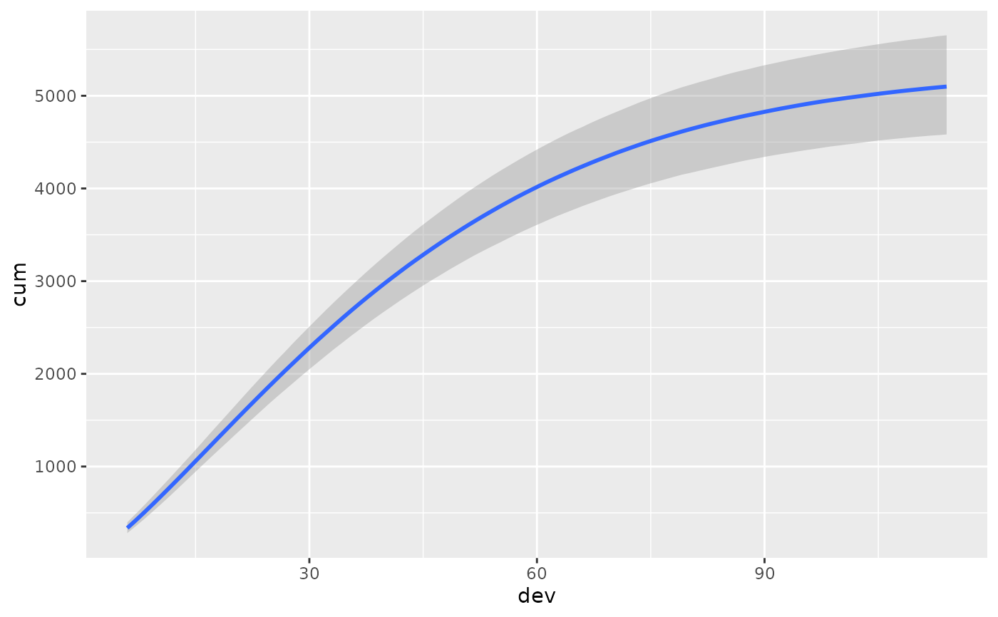 # Normal model with heterogeneous variances
data_het <- data.frame(
y = c(rnorm(50), rnorm(50, 1, 2)),
x = factor(rep(c("a", "b"), each = 50))
)
fit6 <- brm(bf(y ~ x, sigma ~ 0 + x), data = data_het)
#> Compiling Stan program...
#> Start sampling
#>
#> SAMPLING FOR MODEL 'anon_model' NOW (CHAIN 1).
#> Chain 1:
#> Chain 1: Gradient evaluation took 2.2e-05 seconds
#> Chain 1: 1000 transitions using 10 leapfrog steps per transition would take 0.22 seconds.
#> Chain 1: Adjust your expectations accordingly!
#> Chain 1:
#> Chain 1:
#> Chain 1: Iteration: 1 / 2000 [ 0%] (Warmup)
#> Chain 1: Iteration: 200 / 2000 [ 10%] (Warmup)
#> Chain 1: Iteration: 400 / 2000 [ 20%] (Warmup)
#> Chain 1: Iteration: 600 / 2000 [ 30%] (Warmup)
#> Chain 1: Iteration: 800 / 2000 [ 40%] (Warmup)
#> Chain 1: Iteration: 1000 / 2000 [ 50%] (Warmup)
#> Chain 1: Iteration: 1001 / 2000 [ 50%] (Sampling)
#> Chain 1: Iteration: 1200 / 2000 [ 60%] (Sampling)
#> Chain 1: Iteration: 1400 / 2000 [ 70%] (Sampling)
#> Chain 1: Iteration: 1600 / 2000 [ 80%] (Sampling)
#> Chain 1: Iteration: 1800 / 2000 [ 90%] (Sampling)
#> Chain 1: Iteration: 2000 / 2000 [100%] (Sampling)
#> Chain 1:
#> Chain 1: Elapsed Time: 0.096 seconds (Warm-up)
#> Chain 1: 0.096 seconds (Sampling)
#> Chain 1: 0.192 seconds (Total)
#> Chain 1:
#>
#> SAMPLING FOR MODEL 'anon_model' NOW (CHAIN 2).
#> Chain 2:
#> Chain 2: Gradient evaluation took 1.5e-05 seconds
#> Chain 2: 1000 transitions using 10 leapfrog steps per transition would take 0.15 seconds.
#> Chain 2: Adjust your expectations accordingly!
#> Chain 2:
#> Chain 2:
#> Chain 2: Iteration: 1 / 2000 [ 0%] (Warmup)
#> Chain 2: Iteration: 200 / 2000 [ 10%] (Warmup)
#> Chain 2: Iteration: 400 / 2000 [ 20%] (Warmup)
#> Chain 2: Iteration: 600 / 2000 [ 30%] (Warmup)
#> Chain 2: Iteration: 800 / 2000 [ 40%] (Warmup)
#> Chain 2: Iteration: 1000 / 2000 [ 50%] (Warmup)
#> Chain 2: Iteration: 1001 / 2000 [ 50%] (Sampling)
#> Chain 2: Iteration: 1200 / 2000 [ 60%] (Sampling)
#> Chain 2: Iteration: 1400 / 2000 [ 70%] (Sampling)
#> Chain 2: Iteration: 1600 / 2000 [ 80%] (Sampling)
#> Chain 2: Iteration: 1800 / 2000 [ 90%] (Sampling)
#> Chain 2: Iteration: 2000 / 2000 [100%] (Sampling)
#> Chain 2:
#> Chain 2: Elapsed Time: 0.095 seconds (Warm-up)
#> Chain 2: 0.098 seconds (Sampling)
#> Chain 2: 0.193 seconds (Total)
#> Chain 2:
#>
#> SAMPLING FOR MODEL 'anon_model' NOW (CHAIN 3).
#> Chain 3:
#> Chain 3: Gradient evaluation took 1.5e-05 seconds
#> Chain 3: 1000 transitions using 10 leapfrog steps per transition would take 0.15 seconds.
#> Chain 3: Adjust your expectations accordingly!
#> Chain 3:
#> Chain 3:
#> Chain 3: Iteration: 1 / 2000 [ 0%] (Warmup)
#> Chain 3: Iteration: 200 / 2000 [ 10%] (Warmup)
#> Chain 3: Iteration: 400 / 2000 [ 20%] (Warmup)
#> Chain 3: Iteration: 600 / 2000 [ 30%] (Warmup)
#> Chain 3: Iteration: 800 / 2000 [ 40%] (Warmup)
#> Chain 3: Iteration: 1000 / 2000 [ 50%] (Warmup)
#> Chain 3: Iteration: 1001 / 2000 [ 50%] (Sampling)
#> Chain 3: Iteration: 1200 / 2000 [ 60%] (Sampling)
#> Chain 3: Iteration: 1400 / 2000 [ 70%] (Sampling)
#> Chain 3: Iteration: 1600 / 2000 [ 80%] (Sampling)
#> Chain 3: Iteration: 1800 / 2000 [ 90%] (Sampling)
#> Chain 3: Iteration: 2000 / 2000 [100%] (Sampling)
#> Chain 3:
#> Chain 3: Elapsed Time: 0.101 seconds (Warm-up)
#> Chain 3: 0.083 seconds (Sampling)
#> Chain 3: 0.184 seconds (Total)
#> Chain 3:
#>
#> SAMPLING FOR MODEL 'anon_model' NOW (CHAIN 4).
#> Chain 4:
#> Chain 4: Gradient evaluation took 1.5e-05 seconds
#> Chain 4: 1000 transitions using 10 leapfrog steps per transition would take 0.15 seconds.
#> Chain 4: Adjust your expectations accordingly!
#> Chain 4:
#> Chain 4:
#> Chain 4: Iteration: 1 / 2000 [ 0%] (Warmup)
#> Chain 4: Iteration: 200 / 2000 [ 10%] (Warmup)
#> Chain 4: Iteration: 400 / 2000 [ 20%] (Warmup)
#> Chain 4: Iteration: 600 / 2000 [ 30%] (Warmup)
#> Chain 4: Iteration: 800 / 2000 [ 40%] (Warmup)
#> Chain 4: Iteration: 1000 / 2000 [ 50%] (Warmup)
#> Chain 4: Iteration: 1001 / 2000 [ 50%] (Sampling)
#> Chain 4: Iteration: 1200 / 2000 [ 60%] (Sampling)
#> Chain 4: Iteration: 1400 / 2000 [ 70%] (Sampling)
#> Chain 4: Iteration: 1600 / 2000 [ 80%] (Sampling)
#> Chain 4: Iteration: 1800 / 2000 [ 90%] (Sampling)
#> Chain 4: Iteration: 2000 / 2000 [100%] (Sampling)
#> Chain 4:
#> Chain 4: Elapsed Time: 0.096 seconds (Warm-up)
#> Chain 4: 0.101 seconds (Sampling)
#> Chain 4: 0.197 seconds (Total)
#> Chain 4:
summary(fit6)
#> Family: gaussian
#> Links: mu = identity; sigma = log
#> Formula: y ~ x
#> sigma ~ 0 + x
#> Data: data_het (Number of observations: 100)
#> Draws: 4 chains, each with iter = 2000; warmup = 1000; thin = 1;
#> total post-warmup draws = 4000
#>
#> Regression Coefficients:
#> Estimate Est.Error l-95% CI u-95% CI Rhat Bulk_ESS Tail_ESS
#> Intercept -0.08 0.14 -0.35 0.19 1.00 5924 3099
#> xb 1.20 0.34 0.53 1.84 1.00 2878 2354
#> sigma_xa -0.04 0.10 -0.22 0.17 1.00 3358 2775
#> sigma_xb 0.75 0.10 0.56 0.97 1.00 3747 2097
#>
#> Draws were sampled using sampling(NUTS). For each parameter, Bulk_ESS
#> and Tail_ESS are effective sample size measures, and Rhat is the potential
#> scale reduction factor on split chains (at convergence, Rhat = 1).
plot(fit6)
# Normal model with heterogeneous variances
data_het <- data.frame(
y = c(rnorm(50), rnorm(50, 1, 2)),
x = factor(rep(c("a", "b"), each = 50))
)
fit6 <- brm(bf(y ~ x, sigma ~ 0 + x), data = data_het)
#> Compiling Stan program...
#> Start sampling
#>
#> SAMPLING FOR MODEL 'anon_model' NOW (CHAIN 1).
#> Chain 1:
#> Chain 1: Gradient evaluation took 2.2e-05 seconds
#> Chain 1: 1000 transitions using 10 leapfrog steps per transition would take 0.22 seconds.
#> Chain 1: Adjust your expectations accordingly!
#> Chain 1:
#> Chain 1:
#> Chain 1: Iteration: 1 / 2000 [ 0%] (Warmup)
#> Chain 1: Iteration: 200 / 2000 [ 10%] (Warmup)
#> Chain 1: Iteration: 400 / 2000 [ 20%] (Warmup)
#> Chain 1: Iteration: 600 / 2000 [ 30%] (Warmup)
#> Chain 1: Iteration: 800 / 2000 [ 40%] (Warmup)
#> Chain 1: Iteration: 1000 / 2000 [ 50%] (Warmup)
#> Chain 1: Iteration: 1001 / 2000 [ 50%] (Sampling)
#> Chain 1: Iteration: 1200 / 2000 [ 60%] (Sampling)
#> Chain 1: Iteration: 1400 / 2000 [ 70%] (Sampling)
#> Chain 1: Iteration: 1600 / 2000 [ 80%] (Sampling)
#> Chain 1: Iteration: 1800 / 2000 [ 90%] (Sampling)
#> Chain 1: Iteration: 2000 / 2000 [100%] (Sampling)
#> Chain 1:
#> Chain 1: Elapsed Time: 0.096 seconds (Warm-up)
#> Chain 1: 0.096 seconds (Sampling)
#> Chain 1: 0.192 seconds (Total)
#> Chain 1:
#>
#> SAMPLING FOR MODEL 'anon_model' NOW (CHAIN 2).
#> Chain 2:
#> Chain 2: Gradient evaluation took 1.5e-05 seconds
#> Chain 2: 1000 transitions using 10 leapfrog steps per transition would take 0.15 seconds.
#> Chain 2: Adjust your expectations accordingly!
#> Chain 2:
#> Chain 2:
#> Chain 2: Iteration: 1 / 2000 [ 0%] (Warmup)
#> Chain 2: Iteration: 200 / 2000 [ 10%] (Warmup)
#> Chain 2: Iteration: 400 / 2000 [ 20%] (Warmup)
#> Chain 2: Iteration: 600 / 2000 [ 30%] (Warmup)
#> Chain 2: Iteration: 800 / 2000 [ 40%] (Warmup)
#> Chain 2: Iteration: 1000 / 2000 [ 50%] (Warmup)
#> Chain 2: Iteration: 1001 / 2000 [ 50%] (Sampling)
#> Chain 2: Iteration: 1200 / 2000 [ 60%] (Sampling)
#> Chain 2: Iteration: 1400 / 2000 [ 70%] (Sampling)
#> Chain 2: Iteration: 1600 / 2000 [ 80%] (Sampling)
#> Chain 2: Iteration: 1800 / 2000 [ 90%] (Sampling)
#> Chain 2: Iteration: 2000 / 2000 [100%] (Sampling)
#> Chain 2:
#> Chain 2: Elapsed Time: 0.095 seconds (Warm-up)
#> Chain 2: 0.098 seconds (Sampling)
#> Chain 2: 0.193 seconds (Total)
#> Chain 2:
#>
#> SAMPLING FOR MODEL 'anon_model' NOW (CHAIN 3).
#> Chain 3:
#> Chain 3: Gradient evaluation took 1.5e-05 seconds
#> Chain 3: 1000 transitions using 10 leapfrog steps per transition would take 0.15 seconds.
#> Chain 3: Adjust your expectations accordingly!
#> Chain 3:
#> Chain 3:
#> Chain 3: Iteration: 1 / 2000 [ 0%] (Warmup)
#> Chain 3: Iteration: 200 / 2000 [ 10%] (Warmup)
#> Chain 3: Iteration: 400 / 2000 [ 20%] (Warmup)
#> Chain 3: Iteration: 600 / 2000 [ 30%] (Warmup)
#> Chain 3: Iteration: 800 / 2000 [ 40%] (Warmup)
#> Chain 3: Iteration: 1000 / 2000 [ 50%] (Warmup)
#> Chain 3: Iteration: 1001 / 2000 [ 50%] (Sampling)
#> Chain 3: Iteration: 1200 / 2000 [ 60%] (Sampling)
#> Chain 3: Iteration: 1400 / 2000 [ 70%] (Sampling)
#> Chain 3: Iteration: 1600 / 2000 [ 80%] (Sampling)
#> Chain 3: Iteration: 1800 / 2000 [ 90%] (Sampling)
#> Chain 3: Iteration: 2000 / 2000 [100%] (Sampling)
#> Chain 3:
#> Chain 3: Elapsed Time: 0.101 seconds (Warm-up)
#> Chain 3: 0.083 seconds (Sampling)
#> Chain 3: 0.184 seconds (Total)
#> Chain 3:
#>
#> SAMPLING FOR MODEL 'anon_model' NOW (CHAIN 4).
#> Chain 4:
#> Chain 4: Gradient evaluation took 1.5e-05 seconds
#> Chain 4: 1000 transitions using 10 leapfrog steps per transition would take 0.15 seconds.
#> Chain 4: Adjust your expectations accordingly!
#> Chain 4:
#> Chain 4:
#> Chain 4: Iteration: 1 / 2000 [ 0%] (Warmup)
#> Chain 4: Iteration: 200 / 2000 [ 10%] (Warmup)
#> Chain 4: Iteration: 400 / 2000 [ 20%] (Warmup)
#> Chain 4: Iteration: 600 / 2000 [ 30%] (Warmup)
#> Chain 4: Iteration: 800 / 2000 [ 40%] (Warmup)
#> Chain 4: Iteration: 1000 / 2000 [ 50%] (Warmup)
#> Chain 4: Iteration: 1001 / 2000 [ 50%] (Sampling)
#> Chain 4: Iteration: 1200 / 2000 [ 60%] (Sampling)
#> Chain 4: Iteration: 1400 / 2000 [ 70%] (Sampling)
#> Chain 4: Iteration: 1600 / 2000 [ 80%] (Sampling)
#> Chain 4: Iteration: 1800 / 2000 [ 90%] (Sampling)
#> Chain 4: Iteration: 2000 / 2000 [100%] (Sampling)
#> Chain 4:
#> Chain 4: Elapsed Time: 0.096 seconds (Warm-up)
#> Chain 4: 0.101 seconds (Sampling)
#> Chain 4: 0.197 seconds (Total)
#> Chain 4:
summary(fit6)
#> Family: gaussian
#> Links: mu = identity; sigma = log
#> Formula: y ~ x
#> sigma ~ 0 + x
#> Data: data_het (Number of observations: 100)
#> Draws: 4 chains, each with iter = 2000; warmup = 1000; thin = 1;
#> total post-warmup draws = 4000
#>
#> Regression Coefficients:
#> Estimate Est.Error l-95% CI u-95% CI Rhat Bulk_ESS Tail_ESS
#> Intercept -0.08 0.14 -0.35 0.19 1.00 5924 3099
#> xb 1.20 0.34 0.53 1.84 1.00 2878 2354
#> sigma_xa -0.04 0.10 -0.22 0.17 1.00 3358 2775
#> sigma_xb 0.75 0.10 0.56 0.97 1.00 3747 2097
#>
#> Draws were sampled using sampling(NUTS). For each parameter, Bulk_ESS
#> and Tail_ESS are effective sample size measures, and Rhat is the potential
#> scale reduction factor on split chains (at convergence, Rhat = 1).
plot(fit6)
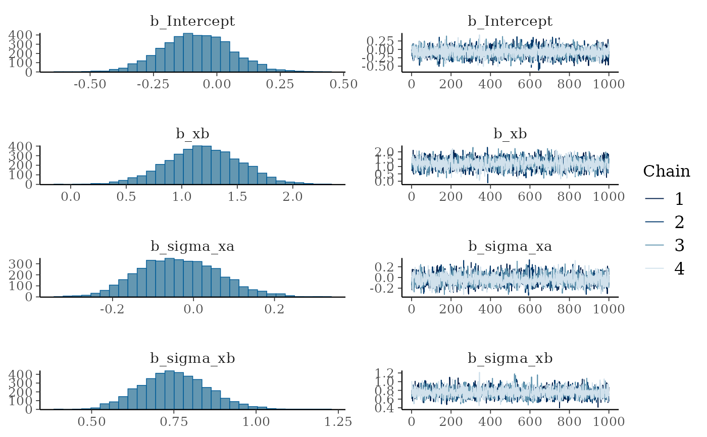 conditional_effects(fit6)
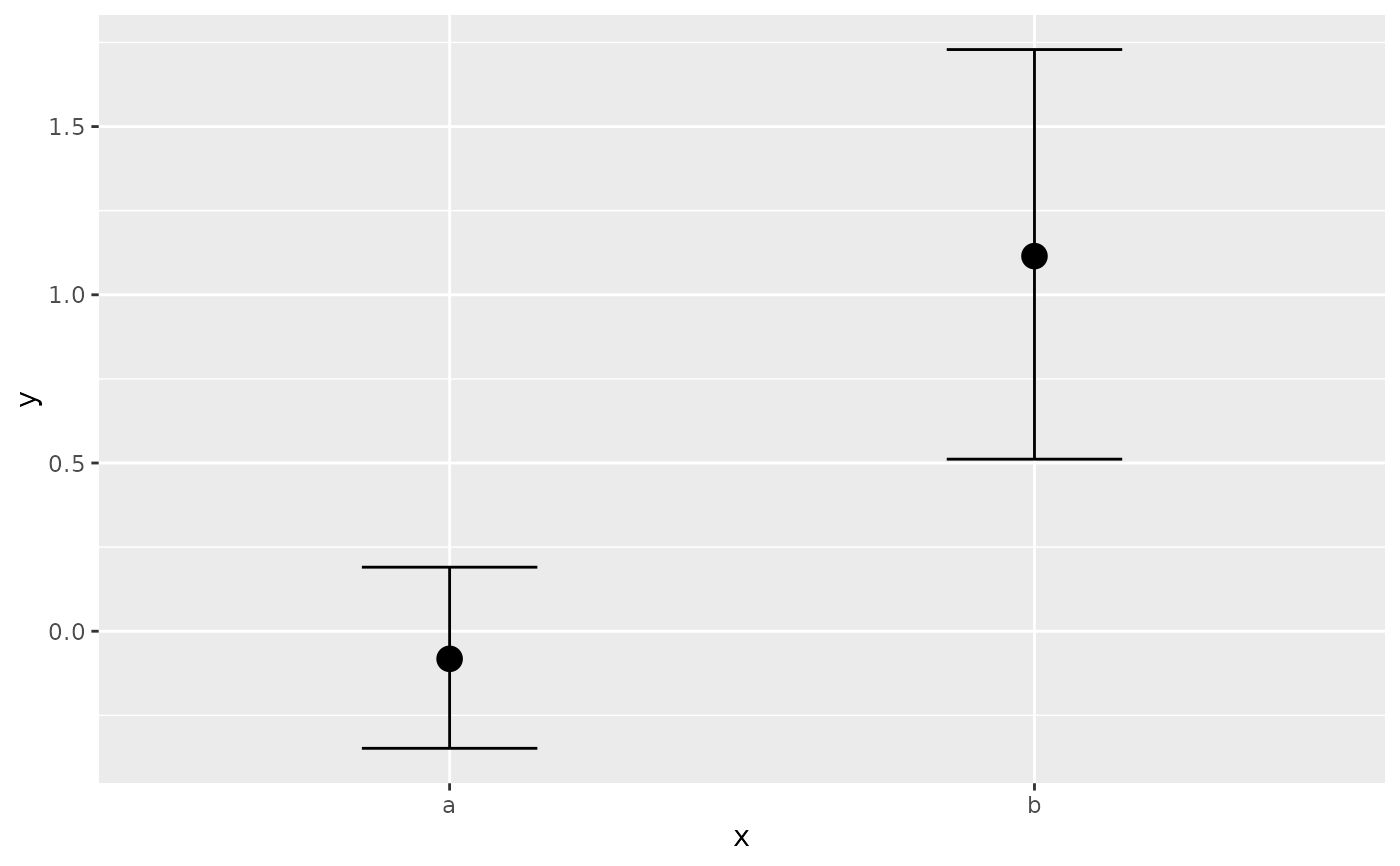 # extract estimated residual SDs of both groups
sigmas <- exp(as.data.frame(fit6, variable = "^b_sigma_", regex = TRUE))
ggplot(stack(sigmas), aes(values)) +
geom_density(aes(fill = ind))
#> Error in ggplot(stack(sigmas), aes(values)): could not find function "ggplot"
# Quantile regression predicting the 25%-quantile
fit7 <- brm(bf(y ~ x, quantile = 0.25), data = data_het,
family = asym_laplace())
#> Compiling Stan program...
#> Start sampling
#>
#> SAMPLING FOR MODEL 'anon_model' NOW (CHAIN 1).
#> Chain 1:
#> Chain 1: Gradient evaluation took 4.1e-05 seconds
#> Chain 1: 1000 transitions using 10 leapfrog steps per transition would take 0.41 seconds.
#> Chain 1: Adjust your expectations accordingly!
#> Chain 1:
#> Chain 1:
#> Chain 1: Iteration: 1 / 2000 [ 0%] (Warmup)
#> Chain 1: Iteration: 200 / 2000 [ 10%] (Warmup)
#> Chain 1: Iteration: 400 / 2000 [ 20%] (Warmup)
#> Chain 1: Iteration: 600 / 2000 [ 30%] (Warmup)
#> Chain 1: Iteration: 800 / 2000 [ 40%] (Warmup)
#> Chain 1: Iteration: 1000 / 2000 [ 50%] (Warmup)
#> Chain 1: Iteration: 1001 / 2000 [ 50%] (Sampling)
#> Chain 1: Iteration: 1200 / 2000 [ 60%] (Sampling)
#> Chain 1: Iteration: 1400 / 2000 [ 70%] (Sampling)
#> Chain 1: Iteration: 1600 / 2000 [ 80%] (Sampling)
#> Chain 1: Iteration: 1800 / 2000 [ 90%] (Sampling)
#> Chain 1: Iteration: 2000 / 2000 [100%] (Sampling)
#> Chain 1:
#> Chain 1: Elapsed Time: 0.209 seconds (Warm-up)
#> Chain 1: 0.225 seconds (Sampling)
#> Chain 1: 0.434 seconds (Total)
#> Chain 1:
#>
#> SAMPLING FOR MODEL 'anon_model' NOW (CHAIN 2).
#> Chain 2:
#> Chain 2: Gradient evaluation took 3.3e-05 seconds
#> Chain 2: 1000 transitions using 10 leapfrog steps per transition would take 0.33 seconds.
#> Chain 2: Adjust your expectations accordingly!
#> Chain 2:
#> Chain 2:
#> Chain 2: Iteration: 1 / 2000 [ 0%] (Warmup)
#> Chain 2: Iteration: 200 / 2000 [ 10%] (Warmup)
#> Chain 2: Iteration: 400 / 2000 [ 20%] (Warmup)
#> Chain 2: Iteration: 600 / 2000 [ 30%] (Warmup)
#> Chain 2: Iteration: 800 / 2000 [ 40%] (Warmup)
#> Chain 2: Iteration: 1000 / 2000 [ 50%] (Warmup)
#> Chain 2: Iteration: 1001 / 2000 [ 50%] (Sampling)
#> Chain 2: Iteration: 1200 / 2000 [ 60%] (Sampling)
#> Chain 2: Iteration: 1400 / 2000 [ 70%] (Sampling)
#> Chain 2: Iteration: 1600 / 2000 [ 80%] (Sampling)
#> Chain 2: Iteration: 1800 / 2000 [ 90%] (Sampling)
#> Chain 2: Iteration: 2000 / 2000 [100%] (Sampling)
#> Chain 2:
#> Chain 2: Elapsed Time: 0.21 seconds (Warm-up)
#> Chain 2: 0.219 seconds (Sampling)
#> Chain 2: 0.429 seconds (Total)
#> Chain 2:
#>
#> SAMPLING FOR MODEL 'anon_model' NOW (CHAIN 3).
#> Chain 3:
#> Chain 3: Gradient evaluation took 3.4e-05 seconds
#> Chain 3: 1000 transitions using 10 leapfrog steps per transition would take 0.34 seconds.
#> Chain 3: Adjust your expectations accordingly!
#> Chain 3:
#> Chain 3:
#> Chain 3: Iteration: 1 / 2000 [ 0%] (Warmup)
#> Chain 3: Iteration: 200 / 2000 [ 10%] (Warmup)
#> Chain 3: Iteration: 400 / 2000 [ 20%] (Warmup)
#> Chain 3: Iteration: 600 / 2000 [ 30%] (Warmup)
#> Chain 3: Iteration: 800 / 2000 [ 40%] (Warmup)
#> Chain 3: Iteration: 1000 / 2000 [ 50%] (Warmup)
#> Chain 3: Iteration: 1001 / 2000 [ 50%] (Sampling)
#> Chain 3: Iteration: 1200 / 2000 [ 60%] (Sampling)
#> Chain 3: Iteration: 1400 / 2000 [ 70%] (Sampling)
#> Chain 3: Iteration: 1600 / 2000 [ 80%] (Sampling)
#> Chain 3: Iteration: 1800 / 2000 [ 90%] (Sampling)
#> Chain 3: Iteration: 2000 / 2000 [100%] (Sampling)
#> Chain 3:
#> Chain 3: Elapsed Time: 0.205 seconds (Warm-up)
#> Chain 3: 0.209 seconds (Sampling)
#> Chain 3: 0.414 seconds (Total)
#> Chain 3:
#>
#> SAMPLING FOR MODEL 'anon_model' NOW (CHAIN 4).
#> Chain 4:
#> Chain 4: Gradient evaluation took 3.4e-05 seconds
#> Chain 4: 1000 transitions using 10 leapfrog steps per transition would take 0.34 seconds.
#> Chain 4: Adjust your expectations accordingly!
#> Chain 4:
#> Chain 4:
#> Chain 4: Iteration: 1 / 2000 [ 0%] (Warmup)
#> Chain 4: Iteration: 200 / 2000 [ 10%] (Warmup)
#> Chain 4: Iteration: 400 / 2000 [ 20%] (Warmup)
#> Chain 4: Iteration: 600 / 2000 [ 30%] (Warmup)
#> Chain 4: Iteration: 800 / 2000 [ 40%] (Warmup)
#> Chain 4: Iteration: 1000 / 2000 [ 50%] (Warmup)
#> Chain 4: Iteration: 1001 / 2000 [ 50%] (Sampling)
#> Chain 4: Iteration: 1200 / 2000 [ 60%] (Sampling)
#> Chain 4: Iteration: 1400 / 2000 [ 70%] (Sampling)
#> Chain 4: Iteration: 1600 / 2000 [ 80%] (Sampling)
#> Chain 4: Iteration: 1800 / 2000 [ 90%] (Sampling)
#> Chain 4: Iteration: 2000 / 2000 [100%] (Sampling)
#> Chain 4:
#> Chain 4: Elapsed Time: 0.219 seconds (Warm-up)
#> Chain 4: 0.211 seconds (Sampling)
#> Chain 4: 0.43 seconds (Total)
#> Chain 4:
summary(fit7)
#> Family: asym_laplace
#> Links: mu = identity
#> Formula: y ~ x
#> quantile = 0.25
#> Data: data_het (Number of observations: 100)
#> Draws: 4 chains, each with iter = 2000; warmup = 1000; thin = 1;
#> total post-warmup draws = 4000
#>
#> Regression Coefficients:
#> Estimate Est.Error l-95% CI u-95% CI Rhat Bulk_ESS Tail_ESS
#> Intercept -0.77 0.15 -1.07 -0.47 1.00 3754 3031
#> xb 0.72 0.30 0.12 1.29 1.00 2291 2289
#>
#> Further Distributional Parameters:
#> Estimate Est.Error l-95% CI u-95% CI Rhat Bulk_ESS Tail_ESS
#> sigma 0.50 0.05 0.41 0.61 1.00 2795 2543
#> quantile 0.25 0.00 0.25 0.25 NA NA NA
#>
#> Draws were sampled using sampling(NUTS). For each parameter, Bulk_ESS
#> and Tail_ESS are effective sample size measures, and Rhat is the potential
#> scale reduction factor on split chains (at convergence, Rhat = 1).
conditional_effects(fit7)
# extract estimated residual SDs of both groups
sigmas <- exp(as.data.frame(fit6, variable = "^b_sigma_", regex = TRUE))
ggplot(stack(sigmas), aes(values)) +
geom_density(aes(fill = ind))
#> Error in ggplot(stack(sigmas), aes(values)): could not find function "ggplot"
# Quantile regression predicting the 25%-quantile
fit7 <- brm(bf(y ~ x, quantile = 0.25), data = data_het,
family = asym_laplace())
#> Compiling Stan program...
#> Start sampling
#>
#> SAMPLING FOR MODEL 'anon_model' NOW (CHAIN 1).
#> Chain 1:
#> Chain 1: Gradient evaluation took 4.1e-05 seconds
#> Chain 1: 1000 transitions using 10 leapfrog steps per transition would take 0.41 seconds.
#> Chain 1: Adjust your expectations accordingly!
#> Chain 1:
#> Chain 1:
#> Chain 1: Iteration: 1 / 2000 [ 0%] (Warmup)
#> Chain 1: Iteration: 200 / 2000 [ 10%] (Warmup)
#> Chain 1: Iteration: 400 / 2000 [ 20%] (Warmup)
#> Chain 1: Iteration: 600 / 2000 [ 30%] (Warmup)
#> Chain 1: Iteration: 800 / 2000 [ 40%] (Warmup)
#> Chain 1: Iteration: 1000 / 2000 [ 50%] (Warmup)
#> Chain 1: Iteration: 1001 / 2000 [ 50%] (Sampling)
#> Chain 1: Iteration: 1200 / 2000 [ 60%] (Sampling)
#> Chain 1: Iteration: 1400 / 2000 [ 70%] (Sampling)
#> Chain 1: Iteration: 1600 / 2000 [ 80%] (Sampling)
#> Chain 1: Iteration: 1800 / 2000 [ 90%] (Sampling)
#> Chain 1: Iteration: 2000 / 2000 [100%] (Sampling)
#> Chain 1:
#> Chain 1: Elapsed Time: 0.209 seconds (Warm-up)
#> Chain 1: 0.225 seconds (Sampling)
#> Chain 1: 0.434 seconds (Total)
#> Chain 1:
#>
#> SAMPLING FOR MODEL 'anon_model' NOW (CHAIN 2).
#> Chain 2:
#> Chain 2: Gradient evaluation took 3.3e-05 seconds
#> Chain 2: 1000 transitions using 10 leapfrog steps per transition would take 0.33 seconds.
#> Chain 2: Adjust your expectations accordingly!
#> Chain 2:
#> Chain 2:
#> Chain 2: Iteration: 1 / 2000 [ 0%] (Warmup)
#> Chain 2: Iteration: 200 / 2000 [ 10%] (Warmup)
#> Chain 2: Iteration: 400 / 2000 [ 20%] (Warmup)
#> Chain 2: Iteration: 600 / 2000 [ 30%] (Warmup)
#> Chain 2: Iteration: 800 / 2000 [ 40%] (Warmup)
#> Chain 2: Iteration: 1000 / 2000 [ 50%] (Warmup)
#> Chain 2: Iteration: 1001 / 2000 [ 50%] (Sampling)
#> Chain 2: Iteration: 1200 / 2000 [ 60%] (Sampling)
#> Chain 2: Iteration: 1400 / 2000 [ 70%] (Sampling)
#> Chain 2: Iteration: 1600 / 2000 [ 80%] (Sampling)
#> Chain 2: Iteration: 1800 / 2000 [ 90%] (Sampling)
#> Chain 2: Iteration: 2000 / 2000 [100%] (Sampling)
#> Chain 2:
#> Chain 2: Elapsed Time: 0.21 seconds (Warm-up)
#> Chain 2: 0.219 seconds (Sampling)
#> Chain 2: 0.429 seconds (Total)
#> Chain 2:
#>
#> SAMPLING FOR MODEL 'anon_model' NOW (CHAIN 3).
#> Chain 3:
#> Chain 3: Gradient evaluation took 3.4e-05 seconds
#> Chain 3: 1000 transitions using 10 leapfrog steps per transition would take 0.34 seconds.
#> Chain 3: Adjust your expectations accordingly!
#> Chain 3:
#> Chain 3:
#> Chain 3: Iteration: 1 / 2000 [ 0%] (Warmup)
#> Chain 3: Iteration: 200 / 2000 [ 10%] (Warmup)
#> Chain 3: Iteration: 400 / 2000 [ 20%] (Warmup)
#> Chain 3: Iteration: 600 / 2000 [ 30%] (Warmup)
#> Chain 3: Iteration: 800 / 2000 [ 40%] (Warmup)
#> Chain 3: Iteration: 1000 / 2000 [ 50%] (Warmup)
#> Chain 3: Iteration: 1001 / 2000 [ 50%] (Sampling)
#> Chain 3: Iteration: 1200 / 2000 [ 60%] (Sampling)
#> Chain 3: Iteration: 1400 / 2000 [ 70%] (Sampling)
#> Chain 3: Iteration: 1600 / 2000 [ 80%] (Sampling)
#> Chain 3: Iteration: 1800 / 2000 [ 90%] (Sampling)
#> Chain 3: Iteration: 2000 / 2000 [100%] (Sampling)
#> Chain 3:
#> Chain 3: Elapsed Time: 0.205 seconds (Warm-up)
#> Chain 3: 0.209 seconds (Sampling)
#> Chain 3: 0.414 seconds (Total)
#> Chain 3:
#>
#> SAMPLING FOR MODEL 'anon_model' NOW (CHAIN 4).
#> Chain 4:
#> Chain 4: Gradient evaluation took 3.4e-05 seconds
#> Chain 4: 1000 transitions using 10 leapfrog steps per transition would take 0.34 seconds.
#> Chain 4: Adjust your expectations accordingly!
#> Chain 4:
#> Chain 4:
#> Chain 4: Iteration: 1 / 2000 [ 0%] (Warmup)
#> Chain 4: Iteration: 200 / 2000 [ 10%] (Warmup)
#> Chain 4: Iteration: 400 / 2000 [ 20%] (Warmup)
#> Chain 4: Iteration: 600 / 2000 [ 30%] (Warmup)
#> Chain 4: Iteration: 800 / 2000 [ 40%] (Warmup)
#> Chain 4: Iteration: 1000 / 2000 [ 50%] (Warmup)
#> Chain 4: Iteration: 1001 / 2000 [ 50%] (Sampling)
#> Chain 4: Iteration: 1200 / 2000 [ 60%] (Sampling)
#> Chain 4: Iteration: 1400 / 2000 [ 70%] (Sampling)
#> Chain 4: Iteration: 1600 / 2000 [ 80%] (Sampling)
#> Chain 4: Iteration: 1800 / 2000 [ 90%] (Sampling)
#> Chain 4: Iteration: 2000 / 2000 [100%] (Sampling)
#> Chain 4:
#> Chain 4: Elapsed Time: 0.219 seconds (Warm-up)
#> Chain 4: 0.211 seconds (Sampling)
#> Chain 4: 0.43 seconds (Total)
#> Chain 4:
summary(fit7)
#> Family: asym_laplace
#> Links: mu = identity
#> Formula: y ~ x
#> quantile = 0.25
#> Data: data_het (Number of observations: 100)
#> Draws: 4 chains, each with iter = 2000; warmup = 1000; thin = 1;
#> total post-warmup draws = 4000
#>
#> Regression Coefficients:
#> Estimate Est.Error l-95% CI u-95% CI Rhat Bulk_ESS Tail_ESS
#> Intercept -0.77 0.15 -1.07 -0.47 1.00 3754 3031
#> xb 0.72 0.30 0.12 1.29 1.00 2291 2289
#>
#> Further Distributional Parameters:
#> Estimate Est.Error l-95% CI u-95% CI Rhat Bulk_ESS Tail_ESS
#> sigma 0.50 0.05 0.41 0.61 1.00 2795 2543
#> quantile 0.25 0.00 0.25 0.25 NA NA NA
#>
#> Draws were sampled using sampling(NUTS). For each parameter, Bulk_ESS
#> and Tail_ESS are effective sample size measures, and Rhat is the potential
#> scale reduction factor on split chains (at convergence, Rhat = 1).
conditional_effects(fit7)
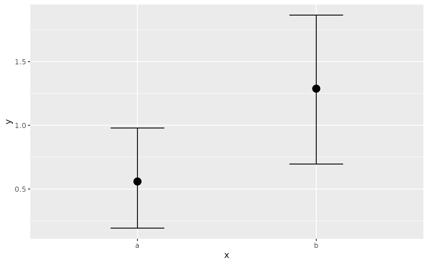 # use the future package for more flexible parallelization
library(future)
plan(multisession, workers = 4)
fit7a <- update(fit7, future = TRUE)
#> Start sampling
#>
#> SAMPLING FOR MODEL 'anon_model' NOW (CHAIN 1).
#> Chain 1:
#> Chain 1: Gradient evaluation took 4.4e-05 seconds
#> Chain 1: 1000 transitions using 10 leapfrog steps per transition would take 0.44 seconds.
#> Chain 1: Adjust your expectations accordingly!
#> Chain 1:
#> Chain 1:
#> Chain 1: Iteration: 1 / 2000 [ 0%] (Warmup)
#> Chain 1: Iteration: 200 / 2000 [ 10%] (Warmup)
#> Chain 1: Iteration: 400 / 2000 [ 20%] (Warmup)
#> Chain 1: Iteration: 600 / 2000 [ 30%] (Warmup)
#> Chain 1: Iteration: 800 / 2000 [ 40%] (Warmup)
#> Chain 1: Iteration: 1000 / 2000 [ 50%] (Warmup)
#> Chain 1: Iteration: 1001 / 2000 [ 50%] (Sampling)
#> Chain 1: Iteration: 1200 / 2000 [ 60%] (Sampling)
#> Chain 1: Iteration: 1400 / 2000 [ 70%] (Sampling)
#> Chain 1: Iteration: 1600 / 2000 [ 80%] (Sampling)
#> Chain 1: Iteration: 1800 / 2000 [ 90%] (Sampling)
#> Chain 1: Iteration: 2000 / 2000 [100%] (Sampling)
#> Chain 1:
#> Chain 1: Elapsed Time: 0.214 seconds (Warm-up)
#> Chain 1: 0.215 seconds (Sampling)
#> Chain 1: 0.429 seconds (Total)
#> Chain 1:
#>
#> SAMPLING FOR MODEL 'anon_model' NOW (CHAIN 2).
#> Chain 2:
#> Chain 2: Gradient evaluation took 4.5e-05 seconds
#> Chain 2: 1000 transitions using 10 leapfrog steps per transition would take 0.45 seconds.
#> Chain 2: Adjust your expectations accordingly!
#> Chain 2:
#> Chain 2:
#> Chain 2: Iteration: 1 / 2000 [ 0%] (Warmup)
#> Chain 2: Iteration: 200 / 2000 [ 10%] (Warmup)
#> Chain 2: Iteration: 400 / 2000 [ 20%] (Warmup)
#> Chain 2: Iteration: 600 / 2000 [ 30%] (Warmup)
#> Chain 2: Iteration: 800 / 2000 [ 40%] (Warmup)
#> Chain 2: Iteration: 1000 / 2000 [ 50%] (Warmup)
#> Chain 2: Iteration: 1001 / 2000 [ 50%] (Sampling)
#> Chain 2: Iteration: 1200 / 2000 [ 60%] (Sampling)
#> Chain 2: Iteration: 1400 / 2000 [ 70%] (Sampling)
#> Chain 2: Iteration: 1600 / 2000 [ 80%] (Sampling)
#> Chain 2: Iteration: 1800 / 2000 [ 90%] (Sampling)
#> Chain 2: Iteration: 2000 / 2000 [100%] (Sampling)
#> Chain 2:
#> Chain 2: Elapsed Time: 0.22 seconds (Warm-up)
#> Chain 2: 0.246 seconds (Sampling)
#> Chain 2: 0.466 seconds (Total)
#> Chain 2:
#>
#> SAMPLING FOR MODEL 'anon_model' NOW (CHAIN 3).
#> Chain 3:
#> Chain 3: Gradient evaluation took 4.2e-05 seconds
#> Chain 3: 1000 transitions using 10 leapfrog steps per transition would take 0.42 seconds.
#> Chain 3: Adjust your expectations accordingly!
#> Chain 3:
#> Chain 3:
#> Chain 3: Iteration: 1 / 2000 [ 0%] (Warmup)
#> Chain 3: Iteration: 200 / 2000 [ 10%] (Warmup)
#> Chain 3: Iteration: 400 / 2000 [ 20%] (Warmup)
#> Chain 3: Iteration: 600 / 2000 [ 30%] (Warmup)
#> Chain 3: Iteration: 800 / 2000 [ 40%] (Warmup)
#> Chain 3: Iteration: 1000 / 2000 [ 50%] (Warmup)
#> Chain 3: Iteration: 1001 / 2000 [ 50%] (Sampling)
#> Chain 3: Iteration: 1200 / 2000 [ 60%] (Sampling)
#> Chain 3: Iteration: 1400 / 2000 [ 70%] (Sampling)
#> Chain 3: Iteration: 1600 / 2000 [ 80%] (Sampling)
#> Chain 3: Iteration: 1800 / 2000 [ 90%] (Sampling)
#> Chain 3: Iteration: 2000 / 2000 [100%] (Sampling)
#> Chain 3:
#> Chain 3: Elapsed Time: 0.217 seconds (Warm-up)
#> Chain 3: 0.21 seconds (Sampling)
#> Chain 3: 0.427 seconds (Total)
#> Chain 3:
#>
#> SAMPLING FOR MODEL 'anon_model' NOW (CHAIN 4).
#> Chain 4:
#> Chain 4: Gradient evaluation took 4.3e-05 seconds
#> Chain 4: 1000 transitions using 10 leapfrog steps per transition would take 0.43 seconds.
#> Chain 4: Adjust your expectations accordingly!
#> Chain 4:
#> Chain 4:
#> Chain 4: Iteration: 1 / 2000 [ 0%] (Warmup)
#> Chain 4: Iteration: 200 / 2000 [ 10%] (Warmup)
#> Chain 4: Iteration: 400 / 2000 [ 20%] (Warmup)
#> Chain 4: Iteration: 600 / 2000 [ 30%] (Warmup)
#> Chain 4: Iteration: 800 / 2000 [ 40%] (Warmup)
#> Chain 4: Iteration: 1000 / 2000 [ 50%] (Warmup)
#> Chain 4: Iteration: 1001 / 2000 [ 50%] (Sampling)
#> Chain 4: Iteration: 1200 / 2000 [ 60%] (Sampling)
#> Chain 4: Iteration: 1400 / 2000 [ 70%] (Sampling)
#> Chain 4: Iteration: 1600 / 2000 [ 80%] (Sampling)
#> Chain 4: Iteration: 1800 / 2000 [ 90%] (Sampling)
#> Chain 4: Iteration: 2000 / 2000 [100%] (Sampling)
#> Chain 4:
#> Chain 4: Elapsed Time: 0.217 seconds (Warm-up)
#> Chain 4: 0.223 seconds (Sampling)
#> Chain 4: 0.44 seconds (Total)
#> Chain 4:
# we may also use mirai allowing the use of remote machines as
# well, including the use of computer clusters managed by queuing
# systems
mirai::daemons(4) # distributed computing with url and remote argument
plan(future.mirai::mirai_cluster)
fit7b <- update(fit7, future = TRUE)
#> Start sampling
#>
#> SAMPLING FOR MODEL 'anon_model' NOW (CHAIN 1).
#> Chain 1:
#> Chain 1: Gradient evaluation took 0.000103 seconds
#> Chain 1: 1000 transitions using 10 leapfrog steps per transition would take 1.03 seconds.
#> Chain 1: Adjust your expectations accordingly!
#> Chain 1:
#> Chain 1:
#> Chain 1: Iteration: 1 / 2000 [ 0%] (Warmup)
#> Chain 1: Iteration: 200 / 2000 [ 10%] (Warmup)
#> Chain 1: Iteration: 400 / 2000 [ 20%] (Warmup)
#> Chain 1: Iteration: 600 / 2000 [ 30%] (Warmup)
#> Chain 1: Iteration: 800 / 2000 [ 40%] (Warmup)
#> Chain 1: Iteration: 1000 / 2000 [ 50%] (Warmup)
#> Chain 1: Iteration: 1001 / 2000 [ 50%] (Sampling)
#> Chain 1: Iteration: 1200 / 2000 [ 60%] (Sampling)
#> Chain 1: Iteration: 1400 / 2000 [ 70%] (Sampling)
#> Chain 1: Iteration: 1600 / 2000 [ 80%] (Sampling)
#> Chain 1: Iteration: 1800 / 2000 [ 90%] (Sampling)
#> Chain 1: Iteration: 2000 / 2000 [100%] (Sampling)
#> Chain 1:
#> Chain 1: Elapsed Time: 0.327 seconds (Warm-up)
#> Chain 1: 0.276 seconds (Sampling)
#> Chain 1: 0.603 seconds (Total)
#> Chain 1:
#>
#> SAMPLING FOR MODEL 'anon_model' NOW (CHAIN 2).
#> Chain 2:
#> Chain 2: Gradient evaluation took 5.2e-05 seconds
#> Chain 2: 1000 transitions using 10 leapfrog steps per transition would take 0.52 seconds.
#> Chain 2: Adjust your expectations accordingly!
#> Chain 2:
#> Chain 2:
#> Chain 2: Iteration: 1 / 2000 [ 0%] (Warmup)
#> Chain 2: Iteration: 200 / 2000 [ 10%] (Warmup)
#> Chain 2: Iteration: 400 / 2000 [ 20%] (Warmup)
#> Chain 2: Iteration: 600 / 2000 [ 30%] (Warmup)
#> Chain 2: Iteration: 800 / 2000 [ 40%] (Warmup)
#> Chain 2: Iteration: 1000 / 2000 [ 50%] (Warmup)
#> Chain 2: Iteration: 1001 / 2000 [ 50%] (Sampling)
#> Chain 2: Iteration: 1200 / 2000 [ 60%] (Sampling)
#> Chain 2: Iteration: 1400 / 2000 [ 70%] (Sampling)
#> Chain 2: Iteration: 1600 / 2000 [ 80%] (Sampling)
#> Chain 2: Iteration: 1800 / 2000 [ 90%] (Sampling)
#> Chain 2: Iteration: 2000 / 2000 [100%] (Sampling)
#> Chain 2:
#> Chain 2: Elapsed Time: 0.287 seconds (Warm-up)
#> Chain 2: 0.263 seconds (Sampling)
#> Chain 2: 0.55 seconds (Total)
#> Chain 2:
#>
#> SAMPLING FOR MODEL 'anon_model' NOW (CHAIN 3).
#> Chain 3:
#> Chain 3: Gradient evaluation took 8.3e-05 seconds
#> Chain 3: 1000 transitions using 10 leapfrog steps per transition would take 0.83 seconds.
#> Chain 3: Adjust your expectations accordingly!
#> Chain 3:
#> Chain 3:
#> Chain 3: Iteration: 1 / 2000 [ 0%] (Warmup)
#> Chain 3: Iteration: 200 / 2000 [ 10%] (Warmup)
#> Chain 3: Iteration: 400 / 2000 [ 20%] (Warmup)
#> Chain 3: Iteration: 600 / 2000 [ 30%] (Warmup)
#> Chain 3: Iteration: 800 / 2000 [ 40%] (Warmup)
#> Chain 3: Iteration: 1000 / 2000 [ 50%] (Warmup)
#> Chain 3: Iteration: 1001 / 2000 [ 50%] (Sampling)
#> Chain 3: Iteration: 1200 / 2000 [ 60%] (Sampling)
#> Chain 3: Iteration: 1400 / 2000 [ 70%] (Sampling)
#> Chain 3: Iteration: 1600 / 2000 [ 80%] (Sampling)
#> Chain 3: Iteration: 1800 / 2000 [ 90%] (Sampling)
#> Chain 3: Iteration: 2000 / 2000 [100%] (Sampling)
#> Chain 3:
#> Chain 3: Elapsed Time: 0.295 seconds (Warm-up)
#> Chain 3: 0.234 seconds (Sampling)
#> Chain 3: 0.529 seconds (Total)
#> Chain 3:
#>
#> SAMPLING FOR MODEL 'anon_model' NOW (CHAIN 4).
#> Chain 4:
#> Chain 4: Gradient evaluation took 5.5e-05 seconds
#> Chain 4: 1000 transitions using 10 leapfrog steps per transition would take 0.55 seconds.
#> Chain 4: Adjust your expectations accordingly!
#> Chain 4:
#> Chain 4:
#> Chain 4: Iteration: 1 / 2000 [ 0%] (Warmup)
#> Chain 4: Iteration: 200 / 2000 [ 10%] (Warmup)
#> Chain 4: Iteration: 400 / 2000 [ 20%] (Warmup)
#> Chain 4: Iteration: 600 / 2000 [ 30%] (Warmup)
#> Chain 4: Iteration: 800 / 2000 [ 40%] (Warmup)
#> Chain 4: Iteration: 1000 / 2000 [ 50%] (Warmup)
#> Chain 4: Iteration: 1001 / 2000 [ 50%] (Sampling)
#> Chain 4: Iteration: 1200 / 2000 [ 60%] (Sampling)
#> Chain 4: Iteration: 1400 / 2000 [ 70%] (Sampling)
#> Chain 4: Iteration: 1600 / 2000 [ 80%] (Sampling)
#> Chain 4: Iteration: 1800 / 2000 [ 90%] (Sampling)
#> Chain 4: Iteration: 2000 / 2000 [100%] (Sampling)
#> Chain 4:
#> Chain 4: Elapsed Time: 0.228 seconds (Warm-up)
#> Chain 4: 0.191 seconds (Sampling)
#> Chain 4: 0.419 seconds (Total)
#> Chain 4:
mirai::daemons(0) # shuts down the 4 workers
# fit a model manually via rstan
scode <- stancode(count ~ Trt, data = epilepsy)
sdata <- standata(count ~ Trt, data = epilepsy)
stanfit <- rstan::stan(model_code = scode, data = sdata)
#>
#> SAMPLING FOR MODEL 'anon_model' NOW (CHAIN 1).
#> Chain 1:
#> Chain 1: Gradient evaluation took 7e-06 seconds
#> Chain 1: 1000 transitions using 10 leapfrog steps per transition would take 0.07 seconds.
#> Chain 1: Adjust your expectations accordingly!
#> Chain 1:
#> Chain 1:
#> Chain 1: Iteration: 1 / 2000 [ 0%] (Warmup)
#> Chain 1: Iteration: 200 / 2000 [ 10%] (Warmup)
#> Chain 1: Iteration: 400 / 2000 [ 20%] (Warmup)
#> Chain 1: Iteration: 600 / 2000 [ 30%] (Warmup)
#> Chain 1: Iteration: 800 / 2000 [ 40%] (Warmup)
#> Chain 1: Iteration: 1000 / 2000 [ 50%] (Warmup)
#> Chain 1: Iteration: 1001 / 2000 [ 50%] (Sampling)
#> Chain 1: Iteration: 1200 / 2000 [ 60%] (Sampling)
#> Chain 1: Iteration: 1400 / 2000 [ 70%] (Sampling)
#> Chain 1: Iteration: 1600 / 2000 [ 80%] (Sampling)
#> Chain 1: Iteration: 1800 / 2000 [ 90%] (Sampling)
#> Chain 1: Iteration: 2000 / 2000 [100%] (Sampling)
#> Chain 1:
#> Chain 1: Elapsed Time: 0.025 seconds (Warm-up)
#> Chain 1: 0.012 seconds (Sampling)
#> Chain 1: 0.037 seconds (Total)
#> Chain 1:
#>
#> SAMPLING FOR MODEL 'anon_model' NOW (CHAIN 2).
#> Chain 2:
#> Chain 2: Gradient evaluation took 3e-06 seconds
#> Chain 2: 1000 transitions using 10 leapfrog steps per transition would take 0.03 seconds.
#> Chain 2: Adjust your expectations accordingly!
#> Chain 2:
#> Chain 2:
#> Chain 2: Iteration: 1 / 2000 [ 0%] (Warmup)
#> Chain 2: Iteration: 200 / 2000 [ 10%] (Warmup)
#> Chain 2: Iteration: 400 / 2000 [ 20%] (Warmup)
#> Chain 2: Iteration: 600 / 2000 [ 30%] (Warmup)
#> Chain 2: Iteration: 800 / 2000 [ 40%] (Warmup)
#> Chain 2: Iteration: 1000 / 2000 [ 50%] (Warmup)
#> Chain 2: Iteration: 1001 / 2000 [ 50%] (Sampling)
#> Chain 2: Iteration: 1200 / 2000 [ 60%] (Sampling)
#> Chain 2: Iteration: 1400 / 2000 [ 70%] (Sampling)
#> Chain 2: Iteration: 1600 / 2000 [ 80%] (Sampling)
#> Chain 2: Iteration: 1800 / 2000 [ 90%] (Sampling)
#> Chain 2: Iteration: 2000 / 2000 [100%] (Sampling)
#> Chain 2:
#> Chain 2: Elapsed Time: 0.023 seconds (Warm-up)
#> Chain 2: 0.013 seconds (Sampling)
#> Chain 2: 0.036 seconds (Total)
#> Chain 2:
#>
#> SAMPLING FOR MODEL 'anon_model' NOW (CHAIN 3).
#> Chain 3:
#> Chain 3: Gradient evaluation took 3e-06 seconds
#> Chain 3: 1000 transitions using 10 leapfrog steps per transition would take 0.03 seconds.
#> Chain 3: Adjust your expectations accordingly!
#> Chain 3:
#> Chain 3:
#> Chain 3: Iteration: 1 / 2000 [ 0%] (Warmup)
#> Chain 3: Iteration: 200 / 2000 [ 10%] (Warmup)
#> Chain 3: Iteration: 400 / 2000 [ 20%] (Warmup)
#> Chain 3: Iteration: 600 / 2000 [ 30%] (Warmup)
#> Chain 3: Iteration: 800 / 2000 [ 40%] (Warmup)
#> Chain 3: Iteration: 1000 / 2000 [ 50%] (Warmup)
#> Chain 3: Iteration: 1001 / 2000 [ 50%] (Sampling)
#> Chain 3: Iteration: 1200 / 2000 [ 60%] (Sampling)
#> Chain 3: Iteration: 1400 / 2000 [ 70%] (Sampling)
#> Chain 3: Iteration: 1600 / 2000 [ 80%] (Sampling)
#> Chain 3: Iteration: 1800 / 2000 [ 90%] (Sampling)
#> Chain 3: Iteration: 2000 / 2000 [100%] (Sampling)
#> Chain 3:
#> Chain 3: Elapsed Time: 0.026 seconds (Warm-up)
#> Chain 3: 0.014 seconds (Sampling)
#> Chain 3: 0.04 seconds (Total)
#> Chain 3:
#>
#> SAMPLING FOR MODEL 'anon_model' NOW (CHAIN 4).
#> Chain 4:
#> Chain 4: Gradient evaluation took 3e-06 seconds
#> Chain 4: 1000 transitions using 10 leapfrog steps per transition would take 0.03 seconds.
#> Chain 4: Adjust your expectations accordingly!
#> Chain 4:
#> Chain 4:
#> Chain 4: Iteration: 1 / 2000 [ 0%] (Warmup)
#> Chain 4: Iteration: 200 / 2000 [ 10%] (Warmup)
#> Chain 4: Iteration: 400 / 2000 [ 20%] (Warmup)
#> Chain 4: Iteration: 600 / 2000 [ 30%] (Warmup)
#> Chain 4: Iteration: 800 / 2000 [ 40%] (Warmup)
#> Chain 4: Iteration: 1000 / 2000 [ 50%] (Warmup)
#> Chain 4: Iteration: 1001 / 2000 [ 50%] (Sampling)
#> Chain 4: Iteration: 1200 / 2000 [ 60%] (Sampling)
#> Chain 4: Iteration: 1400 / 2000 [ 70%] (Sampling)
#> Chain 4: Iteration: 1600 / 2000 [ 80%] (Sampling)
#> Chain 4: Iteration: 1800 / 2000 [ 90%] (Sampling)
#> Chain 4: Iteration: 2000 / 2000 [100%] (Sampling)
#> Chain 4:
#> Chain 4: Elapsed Time: 0.023 seconds (Warm-up)
#> Chain 4: 0.014 seconds (Sampling)
#> Chain 4: 0.037 seconds (Total)
#> Chain 4:
# feed the Stan model back into brms
fit8 <- brm(count ~ Trt, data = epilepsy, empty = TRUE)
fit8$fit <- stanfit
fit8 <- rename_pars(fit8)
summary(fit8)
#> Family: gaussian
#> Links: mu = identity
#> Formula: count ~ Trt
#> Data: epilepsy (Number of observations: 236)
#> Draws: 4 chains, each with iter = 2000; warmup = 1000; thin = 1;
#> total post-warmup draws = 4000
#>
#> Regression Coefficients:
#> Estimate Est.Error l-95% CI u-95% CI Rhat Bulk_ESS Tail_ESS
#> Intercept 8.43 1.20 6.09 10.74 1.00 4109 2787
#> Trt1 -0.61 1.65 -3.87 2.61 1.00 4594 2902
#>
#> Further Distributional Parameters:
#> Estimate Est.Error l-95% CI u-95% CI Rhat Bulk_ESS Tail_ESS
#> sigma 12.37 0.56 11.33 13.53 1.00 4671 3366
#>
#> Draws were sampled using sampling(NUTS). For each parameter, Bulk_ESS
#> and Tail_ESS are effective sample size measures, and Rhat is the potential
#> scale reduction factor on split chains (at convergence, Rhat = 1).
# }
# use the future package for more flexible parallelization
library(future)
plan(multisession, workers = 4)
fit7a <- update(fit7, future = TRUE)
#> Start sampling
#>
#> SAMPLING FOR MODEL 'anon_model' NOW (CHAIN 1).
#> Chain 1:
#> Chain 1: Gradient evaluation took 4.4e-05 seconds
#> Chain 1: 1000 transitions using 10 leapfrog steps per transition would take 0.44 seconds.
#> Chain 1: Adjust your expectations accordingly!
#> Chain 1:
#> Chain 1:
#> Chain 1: Iteration: 1 / 2000 [ 0%] (Warmup)
#> Chain 1: Iteration: 200 / 2000 [ 10%] (Warmup)
#> Chain 1: Iteration: 400 / 2000 [ 20%] (Warmup)
#> Chain 1: Iteration: 600 / 2000 [ 30%] (Warmup)
#> Chain 1: Iteration: 800 / 2000 [ 40%] (Warmup)
#> Chain 1: Iteration: 1000 / 2000 [ 50%] (Warmup)
#> Chain 1: Iteration: 1001 / 2000 [ 50%] (Sampling)
#> Chain 1: Iteration: 1200 / 2000 [ 60%] (Sampling)
#> Chain 1: Iteration: 1400 / 2000 [ 70%] (Sampling)
#> Chain 1: Iteration: 1600 / 2000 [ 80%] (Sampling)
#> Chain 1: Iteration: 1800 / 2000 [ 90%] (Sampling)
#> Chain 1: Iteration: 2000 / 2000 [100%] (Sampling)
#> Chain 1:
#> Chain 1: Elapsed Time: 0.214 seconds (Warm-up)
#> Chain 1: 0.215 seconds (Sampling)
#> Chain 1: 0.429 seconds (Total)
#> Chain 1:
#>
#> SAMPLING FOR MODEL 'anon_model' NOW (CHAIN 2).
#> Chain 2:
#> Chain 2: Gradient evaluation took 4.5e-05 seconds
#> Chain 2: 1000 transitions using 10 leapfrog steps per transition would take 0.45 seconds.
#> Chain 2: Adjust your expectations accordingly!
#> Chain 2:
#> Chain 2:
#> Chain 2: Iteration: 1 / 2000 [ 0%] (Warmup)
#> Chain 2: Iteration: 200 / 2000 [ 10%] (Warmup)
#> Chain 2: Iteration: 400 / 2000 [ 20%] (Warmup)
#> Chain 2: Iteration: 600 / 2000 [ 30%] (Warmup)
#> Chain 2: Iteration: 800 / 2000 [ 40%] (Warmup)
#> Chain 2: Iteration: 1000 / 2000 [ 50%] (Warmup)
#> Chain 2: Iteration: 1001 / 2000 [ 50%] (Sampling)
#> Chain 2: Iteration: 1200 / 2000 [ 60%] (Sampling)
#> Chain 2: Iteration: 1400 / 2000 [ 70%] (Sampling)
#> Chain 2: Iteration: 1600 / 2000 [ 80%] (Sampling)
#> Chain 2: Iteration: 1800 / 2000 [ 90%] (Sampling)
#> Chain 2: Iteration: 2000 / 2000 [100%] (Sampling)
#> Chain 2:
#> Chain 2: Elapsed Time: 0.22 seconds (Warm-up)
#> Chain 2: 0.246 seconds (Sampling)
#> Chain 2: 0.466 seconds (Total)
#> Chain 2:
#>
#> SAMPLING FOR MODEL 'anon_model' NOW (CHAIN 3).
#> Chain 3:
#> Chain 3: Gradient evaluation took 4.2e-05 seconds
#> Chain 3: 1000 transitions using 10 leapfrog steps per transition would take 0.42 seconds.
#> Chain 3: Adjust your expectations accordingly!
#> Chain 3:
#> Chain 3:
#> Chain 3: Iteration: 1 / 2000 [ 0%] (Warmup)
#> Chain 3: Iteration: 200 / 2000 [ 10%] (Warmup)
#> Chain 3: Iteration: 400 / 2000 [ 20%] (Warmup)
#> Chain 3: Iteration: 600 / 2000 [ 30%] (Warmup)
#> Chain 3: Iteration: 800 / 2000 [ 40%] (Warmup)
#> Chain 3: Iteration: 1000 / 2000 [ 50%] (Warmup)
#> Chain 3: Iteration: 1001 / 2000 [ 50%] (Sampling)
#> Chain 3: Iteration: 1200 / 2000 [ 60%] (Sampling)
#> Chain 3: Iteration: 1400 / 2000 [ 70%] (Sampling)
#> Chain 3: Iteration: 1600 / 2000 [ 80%] (Sampling)
#> Chain 3: Iteration: 1800 / 2000 [ 90%] (Sampling)
#> Chain 3: Iteration: 2000 / 2000 [100%] (Sampling)
#> Chain 3:
#> Chain 3: Elapsed Time: 0.217 seconds (Warm-up)
#> Chain 3: 0.21 seconds (Sampling)
#> Chain 3: 0.427 seconds (Total)
#> Chain 3:
#>
#> SAMPLING FOR MODEL 'anon_model' NOW (CHAIN 4).
#> Chain 4:
#> Chain 4: Gradient evaluation took 4.3e-05 seconds
#> Chain 4: 1000 transitions using 10 leapfrog steps per transition would take 0.43 seconds.
#> Chain 4: Adjust your expectations accordingly!
#> Chain 4:
#> Chain 4:
#> Chain 4: Iteration: 1 / 2000 [ 0%] (Warmup)
#> Chain 4: Iteration: 200 / 2000 [ 10%] (Warmup)
#> Chain 4: Iteration: 400 / 2000 [ 20%] (Warmup)
#> Chain 4: Iteration: 600 / 2000 [ 30%] (Warmup)
#> Chain 4: Iteration: 800 / 2000 [ 40%] (Warmup)
#> Chain 4: Iteration: 1000 / 2000 [ 50%] (Warmup)
#> Chain 4: Iteration: 1001 / 2000 [ 50%] (Sampling)
#> Chain 4: Iteration: 1200 / 2000 [ 60%] (Sampling)
#> Chain 4: Iteration: 1400 / 2000 [ 70%] (Sampling)
#> Chain 4: Iteration: 1600 / 2000 [ 80%] (Sampling)
#> Chain 4: Iteration: 1800 / 2000 [ 90%] (Sampling)
#> Chain 4: Iteration: 2000 / 2000 [100%] (Sampling)
#> Chain 4:
#> Chain 4: Elapsed Time: 0.217 seconds (Warm-up)
#> Chain 4: 0.223 seconds (Sampling)
#> Chain 4: 0.44 seconds (Total)
#> Chain 4:
# we may also use mirai allowing the use of remote machines as
# well, including the use of computer clusters managed by queuing
# systems
mirai::daemons(4) # distributed computing with url and remote argument
plan(future.mirai::mirai_cluster)
fit7b <- update(fit7, future = TRUE)
#> Start sampling
#>
#> SAMPLING FOR MODEL 'anon_model' NOW (CHAIN 1).
#> Chain 1:
#> Chain 1: Gradient evaluation took 0.000103 seconds
#> Chain 1: 1000 transitions using 10 leapfrog steps per transition would take 1.03 seconds.
#> Chain 1: Adjust your expectations accordingly!
#> Chain 1:
#> Chain 1:
#> Chain 1: Iteration: 1 / 2000 [ 0%] (Warmup)
#> Chain 1: Iteration: 200 / 2000 [ 10%] (Warmup)
#> Chain 1: Iteration: 400 / 2000 [ 20%] (Warmup)
#> Chain 1: Iteration: 600 / 2000 [ 30%] (Warmup)
#> Chain 1: Iteration: 800 / 2000 [ 40%] (Warmup)
#> Chain 1: Iteration: 1000 / 2000 [ 50%] (Warmup)
#> Chain 1: Iteration: 1001 / 2000 [ 50%] (Sampling)
#> Chain 1: Iteration: 1200 / 2000 [ 60%] (Sampling)
#> Chain 1: Iteration: 1400 / 2000 [ 70%] (Sampling)
#> Chain 1: Iteration: 1600 / 2000 [ 80%] (Sampling)
#> Chain 1: Iteration: 1800 / 2000 [ 90%] (Sampling)
#> Chain 1: Iteration: 2000 / 2000 [100%] (Sampling)
#> Chain 1:
#> Chain 1: Elapsed Time: 0.327 seconds (Warm-up)
#> Chain 1: 0.276 seconds (Sampling)
#> Chain 1: 0.603 seconds (Total)
#> Chain 1:
#>
#> SAMPLING FOR MODEL 'anon_model' NOW (CHAIN 2).
#> Chain 2:
#> Chain 2: Gradient evaluation took 5.2e-05 seconds
#> Chain 2: 1000 transitions using 10 leapfrog steps per transition would take 0.52 seconds.
#> Chain 2: Adjust your expectations accordingly!
#> Chain 2:
#> Chain 2:
#> Chain 2: Iteration: 1 / 2000 [ 0%] (Warmup)
#> Chain 2: Iteration: 200 / 2000 [ 10%] (Warmup)
#> Chain 2: Iteration: 400 / 2000 [ 20%] (Warmup)
#> Chain 2: Iteration: 600 / 2000 [ 30%] (Warmup)
#> Chain 2: Iteration: 800 / 2000 [ 40%] (Warmup)
#> Chain 2: Iteration: 1000 / 2000 [ 50%] (Warmup)
#> Chain 2: Iteration: 1001 / 2000 [ 50%] (Sampling)
#> Chain 2: Iteration: 1200 / 2000 [ 60%] (Sampling)
#> Chain 2: Iteration: 1400 / 2000 [ 70%] (Sampling)
#> Chain 2: Iteration: 1600 / 2000 [ 80%] (Sampling)
#> Chain 2: Iteration: 1800 / 2000 [ 90%] (Sampling)
#> Chain 2: Iteration: 2000 / 2000 [100%] (Sampling)
#> Chain 2:
#> Chain 2: Elapsed Time: 0.287 seconds (Warm-up)
#> Chain 2: 0.263 seconds (Sampling)
#> Chain 2: 0.55 seconds (Total)
#> Chain 2:
#>
#> SAMPLING FOR MODEL 'anon_model' NOW (CHAIN 3).
#> Chain 3:
#> Chain 3: Gradient evaluation took 8.3e-05 seconds
#> Chain 3: 1000 transitions using 10 leapfrog steps per transition would take 0.83 seconds.
#> Chain 3: Adjust your expectations accordingly!
#> Chain 3:
#> Chain 3:
#> Chain 3: Iteration: 1 / 2000 [ 0%] (Warmup)
#> Chain 3: Iteration: 200 / 2000 [ 10%] (Warmup)
#> Chain 3: Iteration: 400 / 2000 [ 20%] (Warmup)
#> Chain 3: Iteration: 600 / 2000 [ 30%] (Warmup)
#> Chain 3: Iteration: 800 / 2000 [ 40%] (Warmup)
#> Chain 3: Iteration: 1000 / 2000 [ 50%] (Warmup)
#> Chain 3: Iteration: 1001 / 2000 [ 50%] (Sampling)
#> Chain 3: Iteration: 1200 / 2000 [ 60%] (Sampling)
#> Chain 3: Iteration: 1400 / 2000 [ 70%] (Sampling)
#> Chain 3: Iteration: 1600 / 2000 [ 80%] (Sampling)
#> Chain 3: Iteration: 1800 / 2000 [ 90%] (Sampling)
#> Chain 3: Iteration: 2000 / 2000 [100%] (Sampling)
#> Chain 3:
#> Chain 3: Elapsed Time: 0.295 seconds (Warm-up)
#> Chain 3: 0.234 seconds (Sampling)
#> Chain 3: 0.529 seconds (Total)
#> Chain 3:
#>
#> SAMPLING FOR MODEL 'anon_model' NOW (CHAIN 4).
#> Chain 4:
#> Chain 4: Gradient evaluation took 5.5e-05 seconds
#> Chain 4: 1000 transitions using 10 leapfrog steps per transition would take 0.55 seconds.
#> Chain 4: Adjust your expectations accordingly!
#> Chain 4:
#> Chain 4:
#> Chain 4: Iteration: 1 / 2000 [ 0%] (Warmup)
#> Chain 4: Iteration: 200 / 2000 [ 10%] (Warmup)
#> Chain 4: Iteration: 400 / 2000 [ 20%] (Warmup)
#> Chain 4: Iteration: 600 / 2000 [ 30%] (Warmup)
#> Chain 4: Iteration: 800 / 2000 [ 40%] (Warmup)
#> Chain 4: Iteration: 1000 / 2000 [ 50%] (Warmup)
#> Chain 4: Iteration: 1001 / 2000 [ 50%] (Sampling)
#> Chain 4: Iteration: 1200 / 2000 [ 60%] (Sampling)
#> Chain 4: Iteration: 1400 / 2000 [ 70%] (Sampling)
#> Chain 4: Iteration: 1600 / 2000 [ 80%] (Sampling)
#> Chain 4: Iteration: 1800 / 2000 [ 90%] (Sampling)
#> Chain 4: Iteration: 2000 / 2000 [100%] (Sampling)
#> Chain 4:
#> Chain 4: Elapsed Time: 0.228 seconds (Warm-up)
#> Chain 4: 0.191 seconds (Sampling)
#> Chain 4: 0.419 seconds (Total)
#> Chain 4:
mirai::daemons(0) # shuts down the 4 workers
# fit a model manually via rstan
scode <- stancode(count ~ Trt, data = epilepsy)
sdata <- standata(count ~ Trt, data = epilepsy)
stanfit <- rstan::stan(model_code = scode, data = sdata)
#>
#> SAMPLING FOR MODEL 'anon_model' NOW (CHAIN 1).
#> Chain 1:
#> Chain 1: Gradient evaluation took 7e-06 seconds
#> Chain 1: 1000 transitions using 10 leapfrog steps per transition would take 0.07 seconds.
#> Chain 1: Adjust your expectations accordingly!
#> Chain 1:
#> Chain 1:
#> Chain 1: Iteration: 1 / 2000 [ 0%] (Warmup)
#> Chain 1: Iteration: 200 / 2000 [ 10%] (Warmup)
#> Chain 1: Iteration: 400 / 2000 [ 20%] (Warmup)
#> Chain 1: Iteration: 600 / 2000 [ 30%] (Warmup)
#> Chain 1: Iteration: 800 / 2000 [ 40%] (Warmup)
#> Chain 1: Iteration: 1000 / 2000 [ 50%] (Warmup)
#> Chain 1: Iteration: 1001 / 2000 [ 50%] (Sampling)
#> Chain 1: Iteration: 1200 / 2000 [ 60%] (Sampling)
#> Chain 1: Iteration: 1400 / 2000 [ 70%] (Sampling)
#> Chain 1: Iteration: 1600 / 2000 [ 80%] (Sampling)
#> Chain 1: Iteration: 1800 / 2000 [ 90%] (Sampling)
#> Chain 1: Iteration: 2000 / 2000 [100%] (Sampling)
#> Chain 1:
#> Chain 1: Elapsed Time: 0.025 seconds (Warm-up)
#> Chain 1: 0.012 seconds (Sampling)
#> Chain 1: 0.037 seconds (Total)
#> Chain 1:
#>
#> SAMPLING FOR MODEL 'anon_model' NOW (CHAIN 2).
#> Chain 2:
#> Chain 2: Gradient evaluation took 3e-06 seconds
#> Chain 2: 1000 transitions using 10 leapfrog steps per transition would take 0.03 seconds.
#> Chain 2: Adjust your expectations accordingly!
#> Chain 2:
#> Chain 2:
#> Chain 2: Iteration: 1 / 2000 [ 0%] (Warmup)
#> Chain 2: Iteration: 200 / 2000 [ 10%] (Warmup)
#> Chain 2: Iteration: 400 / 2000 [ 20%] (Warmup)
#> Chain 2: Iteration: 600 / 2000 [ 30%] (Warmup)
#> Chain 2: Iteration: 800 / 2000 [ 40%] (Warmup)
#> Chain 2: Iteration: 1000 / 2000 [ 50%] (Warmup)
#> Chain 2: Iteration: 1001 / 2000 [ 50%] (Sampling)
#> Chain 2: Iteration: 1200 / 2000 [ 60%] (Sampling)
#> Chain 2: Iteration: 1400 / 2000 [ 70%] (Sampling)
#> Chain 2: Iteration: 1600 / 2000 [ 80%] (Sampling)
#> Chain 2: Iteration: 1800 / 2000 [ 90%] (Sampling)
#> Chain 2: Iteration: 2000 / 2000 [100%] (Sampling)
#> Chain 2:
#> Chain 2: Elapsed Time: 0.023 seconds (Warm-up)
#> Chain 2: 0.013 seconds (Sampling)
#> Chain 2: 0.036 seconds (Total)
#> Chain 2:
#>
#> SAMPLING FOR MODEL 'anon_model' NOW (CHAIN 3).
#> Chain 3:
#> Chain 3: Gradient evaluation took 3e-06 seconds
#> Chain 3: 1000 transitions using 10 leapfrog steps per transition would take 0.03 seconds.
#> Chain 3: Adjust your expectations accordingly!
#> Chain 3:
#> Chain 3:
#> Chain 3: Iteration: 1 / 2000 [ 0%] (Warmup)
#> Chain 3: Iteration: 200 / 2000 [ 10%] (Warmup)
#> Chain 3: Iteration: 400 / 2000 [ 20%] (Warmup)
#> Chain 3: Iteration: 600 / 2000 [ 30%] (Warmup)
#> Chain 3: Iteration: 800 / 2000 [ 40%] (Warmup)
#> Chain 3: Iteration: 1000 / 2000 [ 50%] (Warmup)
#> Chain 3: Iteration: 1001 / 2000 [ 50%] (Sampling)
#> Chain 3: Iteration: 1200 / 2000 [ 60%] (Sampling)
#> Chain 3: Iteration: 1400 / 2000 [ 70%] (Sampling)
#> Chain 3: Iteration: 1600 / 2000 [ 80%] (Sampling)
#> Chain 3: Iteration: 1800 / 2000 [ 90%] (Sampling)
#> Chain 3: Iteration: 2000 / 2000 [100%] (Sampling)
#> Chain 3:
#> Chain 3: Elapsed Time: 0.026 seconds (Warm-up)
#> Chain 3: 0.014 seconds (Sampling)
#> Chain 3: 0.04 seconds (Total)
#> Chain 3:
#>
#> SAMPLING FOR MODEL 'anon_model' NOW (CHAIN 4).
#> Chain 4:
#> Chain 4: Gradient evaluation took 3e-06 seconds
#> Chain 4: 1000 transitions using 10 leapfrog steps per transition would take 0.03 seconds.
#> Chain 4: Adjust your expectations accordingly!
#> Chain 4:
#> Chain 4:
#> Chain 4: Iteration: 1 / 2000 [ 0%] (Warmup)
#> Chain 4: Iteration: 200 / 2000 [ 10%] (Warmup)
#> Chain 4: Iteration: 400 / 2000 [ 20%] (Warmup)
#> Chain 4: Iteration: 600 / 2000 [ 30%] (Warmup)
#> Chain 4: Iteration: 800 / 2000 [ 40%] (Warmup)
#> Chain 4: Iteration: 1000 / 2000 [ 50%] (Warmup)
#> Chain 4: Iteration: 1001 / 2000 [ 50%] (Sampling)
#> Chain 4: Iteration: 1200 / 2000 [ 60%] (Sampling)
#> Chain 4: Iteration: 1400 / 2000 [ 70%] (Sampling)
#> Chain 4: Iteration: 1600 / 2000 [ 80%] (Sampling)
#> Chain 4: Iteration: 1800 / 2000 [ 90%] (Sampling)
#> Chain 4: Iteration: 2000 / 2000 [100%] (Sampling)
#> Chain 4:
#> Chain 4: Elapsed Time: 0.023 seconds (Warm-up)
#> Chain 4: 0.014 seconds (Sampling)
#> Chain 4: 0.037 seconds (Total)
#> Chain 4:
# feed the Stan model back into brms
fit8 <- brm(count ~ Trt, data = epilepsy, empty = TRUE)
fit8$fit <- stanfit
fit8 <- rename_pars(fit8)
summary(fit8)
#> Family: gaussian
#> Links: mu = identity
#> Formula: count ~ Trt
#> Data: epilepsy (Number of observations: 236)
#> Draws: 4 chains, each with iter = 2000; warmup = 1000; thin = 1;
#> total post-warmup draws = 4000
#>
#> Regression Coefficients:
#> Estimate Est.Error l-95% CI u-95% CI Rhat Bulk_ESS Tail_ESS
#> Intercept 8.43 1.20 6.09 10.74 1.00 4109 2787
#> Trt1 -0.61 1.65 -3.87 2.61 1.00 4594 2902
#>
#> Further Distributional Parameters:
#> Estimate Est.Error l-95% CI u-95% CI Rhat Bulk_ESS Tail_ESS
#> sigma 12.37 0.56 11.33 13.53 1.00 4671 3366
#>
#> Draws were sampled using sampling(NUTS). For each parameter, Bulk_ESS
#> and Tail_ESS are effective sample size measures, and Rhat is the potential
#> scale reduction factor on split chains (at convergence, Rhat = 1).
# }