
Display Conditional Effects of Predictors
Source:R/conditional_effects.R
conditional_effects.brmsfit.RdDisplay conditional effects of one or more numeric and/or categorical predictors including two-way interaction effects.
Usage
# S3 method for class 'brmsfit'
conditional_effects(
  x,
  effects = NULL,
  conditions = NULL,
  int_conditions = NULL,
  re_formula = NA,
  prob = 0.95,
  robust = TRUE,
  method = "posterior_epred",
  spaghetti = FALSE,
  surface = FALSE,
  categorical = FALSE,
  ordinal = FALSE,
  transform = NULL,
  resolution = 100,
  select_points = 0,
  too_far = 0,
  probs = NULL,
  ...
)

conditional_effects(x, ...)

# S3 method for class 'brms_conditional_effects'
plot(
  x,
  ncol = NULL,
  points = getOption("brms.plot_points", FALSE),
  rug = getOption("brms.plot_rug", FALSE),
  mean = TRUE,
  jitter_width = 0,
  stype = c("contour", "raster"),
  line_args = list(),
  cat_args = list(),
  errorbar_args = list(),
  surface_args = list(),
  spaghetti_args = list(),
  point_args = list(),
  rug_args = list(),
  facet_args = list(),
  theme = NULL,
  ask = TRUE,
  plot = TRUE,
  ...
)
Arguments
- x
An object of class
brmsfit.- effects
An optional character vector naming effects (main effects or interactions) for which to compute conditional plots. Interactions are specified by a
:between variable names. IfNULL(the default), plots are generated for all main effects and two-way interactions estimated in the model. When specifyingeffectsmanually, all two-way interactions (including grouping variables) may be plotted even if not originally modeled.- conditions
An optional
data.framecontaining variable values to condition on. Each effect defined ineffectswill be plotted separately for each row ofconditions. Values in thecond__column will be used as titles of the subplots. Ifcond__is not given, the row names will be used for this purpose instead. It is recommended to only define a few rows in order to keep the plots clear. Seemake_conditionsfor an easy way to define conditions. IfNULL(the default), numeric variables will be conditionalized by using their means and factors will get their first level assigned.NAvalues within factors are interpreted as if all dummy variables of this factor are zero. This allows, for instance, to make predictions of the grand mean when using sum coding.- int_conditions
An optional named
listwhose elements are vectors of values of the variables specified ineffects. At these values, predictions are evaluated. The names ofint_conditionshave to match the variable names exactly. Additionally, the elements of the vectors may be named themselves, in which case their names appear as labels for the conditions in the plots. Instead of vectors, functions returning vectors may be passed and are applied on the original values of the corresponding variable. IfNULL(the default), predictions are evaluated at the \(mean\) and at \(mean +/- sd\) for numeric predictors and at all categories for factor-like predictors.- re_formula
A formula containing group-level effects to be considered in the conditional predictions. If
NULL, include all group-level effects; ifNA(default), include no group-level effects.- prob
A value between 0 and 1 indicating the desired probability to be covered by the uncertainty intervals. The default is 0.95.
- robust
If
TRUE(the default) the median is used as the measure of central tendency. IfFALSEthe mean is used instead.- method
Method used to obtain predictions. Can be set to
"posterior_epred"(the default),"posterior_predict", or"posterior_linpred". For more details, see the respective function documentations.- spaghetti
Logical. Indicates if predictions should be visualized via spaghetti plots. Only applied for numeric predictors. If
TRUE, it is recommended to set argumentndrawsto a relatively small value (e.g.,100) in order to reduce computation time.- surface
Logical. Indicates if interactions or two-dimensional smooths should be visualized as a surface. Defaults to
FALSE. The surface type can be controlled via argumentstypeof the related plotting method.- categorical
Logical. Indicates if effects of categorical or ordinal models should be shown in terms of probabilities of response categories. Defaults to
FALSE.- ordinal
(Deprecated) Please use argument
categorical. Logical. Indicates if effects in ordinal models should be visualized as a raster with the response categories on the y-axis. Defaults toFALSE.- transform
A function or a character string naming a function to be applied on the predicted responses before summary statistics are computed. Only allowed if
method = "posterior_predict".- resolution
Number of support points used to generate the plots. Higher resolution leads to smoother plots. Defaults to
100. IfsurfaceisTRUE, this implies10000support points for interaction terms, so it might be necessary to reduceresolutionwhen only few RAM is available.- select_points
Positive number. Only relevant if
pointsorrugare set toTRUE: Actual data points of numeric variables that are too far away from the values specified inconditionscan be excluded from the plot. Values are scaled into the unit interval and then points more thanselect_pointsfrom the values inconditionsare excluded. By default, all points are used.- too_far
Positive number. For surface plots only: Grid points that are too far away from the actual data points can be excluded from the plot.
too_fardetermines what is too far. The grid is scaled into the unit square and then grid points more thantoo_farfrom the predictor variables are excluded. By default, all grid points are used. Ignored for non-surface plots.- probs
(Deprecated) The quantiles to be used in the computation of uncertainty intervals. Please use argument
probinstead.- ...
Further arguments such as
draw_idsorndrawspassed toposterior_predictorposterior_epred.- ncol
Number of plots to display per column for each effect. If
NULL(default),ncolis computed internally based on the number of rows ofconditions.- points
Logical. Indicates if the original data points should be added via
geom_jitter. Default isFALSE. Can be controlled globally via thebrms.plot_pointsoption. Note that only those data points will be added that match the specified conditions defined inconditions. For categorical predictors, the conditions have to match exactly. For numeric predictors, argumentselect_pointsis used to determine, which points do match a condition.- rug
Logical. Indicates if a rug representation of predictor values should be added via
geom_rug. Default isFALSE. Depends onselect_pointsin the same way aspointsdoes. Can be controlled globally via thebrms.plot_rugoption.- mean
Logical. Only relevant for spaghetti plots. If
TRUE(the default), display the mean regression line on top of the regression lines for each sample.- jitter_width
Only used if
points = TRUE: Amount of horizontal jittering of the data points. Mainly useful for ordinal models. Defaults to0that is no jittering.- stype
Indicates how surface plots should be displayed. Either
"contour"or"raster".- line_args
Only used in plots of continuous predictors: A named list of arguments passed to
geom_smooth.- cat_args
Only used in plots of categorical predictors: A named list of arguments passed to
geom_point.- errorbar_args
Only used in plots of categorical predictors: A named list of arguments passed to
geom_errorbar.- surface_args
Only used in surface plots: A named list of arguments passed to
geom_contourorgeom_raster(depending on argumentstype).- spaghetti_args
Only used in spaghetti plots: A named list of arguments passed to
geom_smooth.- point_args
Only used if
points = TRUE: A named list of arguments passed togeom_jitter.- rug_args
Only used if
rug = TRUE: A named list of arguments passed togeom_rug.- facet_args
Only used if if multiple conditions are provided: A named list of arguments passed to
facet_wrap.- theme
A
themeobject modifying the appearance of the plots. For some basic themes seeggthemeandtheme_default.- ask
Logical; indicates if the user is prompted before a new page is plotted. Only used if
plotisTRUE.- plot
Logical; indicates if plots should be plotted directly in the active graphic device. Defaults to
TRUE.
Value
An object of class 'brms_conditional_effects' which is a
named list with one data.frame per effect containing all information
required to generate conditional effects plots. Among others, these
data.frames contain some special variables, namely estimate__
(predicted values of the response), se__ (standard error of the
predicted response), lower__ and upper__ (lower and upper
bounds of the uncertainty interval of the response), as well as
cond__ (used in faceting when conditions contains multiple
rows).
The corresponding plot method returns a named
list of ggplot objects, which can be further
customized using the ggplot2 package.
Details
When creating conditional_effects for a particular predictor
(or interaction of two predictors), one has to choose the values of all
other predictors to condition on. By default, the mean is used for
continuous variables and the reference category is used for factors, but
you may change these values via argument conditions. This also has
an implication for the points argument: In the created plots, only
those points will be shown that correspond to the factor levels actually
used in the conditioning, in order not to create the false impression of
bad model fit, where it is just due to conditioning on certain factor
levels.
To fully change colors of the created plots, one has to amend both
scale_colour and scale_fill. See
scale_colour_grey or
scale_colour_gradient for
more details.
Examples
# \dontrun{
fit <- brm(count ~ zAge + zBase * Trt + (1 | patient),
data = epilepsy, family = poisson())
#> Compiling Stan program...
#> Start sampling
#>
#> SAMPLING FOR MODEL 'anon_model' NOW (CHAIN 1).
#> Chain 1:
#> Chain 1: Gradient evaluation took 3.2e-05 seconds
#> Chain 1: 1000 transitions using 10 leapfrog steps per transition would take 0.32 seconds.
#> Chain 1: Adjust your expectations accordingly!
#> Chain 1:
#> Chain 1:
#> Chain 1: Iteration: 1 / 2000 [ 0%] (Warmup)
#> Chain 1: Iteration: 200 / 2000 [ 10%] (Warmup)
#> Chain 1: Iteration: 400 / 2000 [ 20%] (Warmup)
#> Chain 1: Iteration: 600 / 2000 [ 30%] (Warmup)
#> Chain 1: Iteration: 800 / 2000 [ 40%] (Warmup)
#> Chain 1: Iteration: 1000 / 2000 [ 50%] (Warmup)
#> Chain 1: Iteration: 1001 / 2000 [ 50%] (Sampling)
#> Chain 1: Iteration: 1200 / 2000 [ 60%] (Sampling)
#> Chain 1: Iteration: 1400 / 2000 [ 70%] (Sampling)
#> Chain 1: Iteration: 1600 / 2000 [ 80%] (Sampling)
#> Chain 1: Iteration: 1800 / 2000 [ 90%] (Sampling)
#> Chain 1: Iteration: 2000 / 2000 [100%] (Sampling)
#> Chain 1:
#> Chain 1: Elapsed Time: 2.088 seconds (Warm-up)
#> Chain 1: 1.431 seconds (Sampling)
#> Chain 1: 3.519 seconds (Total)
#> Chain 1:
#>
#> SAMPLING FOR MODEL 'anon_model' NOW (CHAIN 2).
#> Chain 2:
#> Chain 2: Gradient evaluation took 2.5e-05 seconds
#> Chain 2: 1000 transitions using 10 leapfrog steps per transition would take 0.25 seconds.
#> Chain 2: Adjust your expectations accordingly!
#> Chain 2:
#> Chain 2:
#> Chain 2: Iteration: 1 / 2000 [ 0%] (Warmup)
#> Chain 2: Iteration: 200 / 2000 [ 10%] (Warmup)
#> Chain 2: Iteration: 400 / 2000 [ 20%] (Warmup)
#> Chain 2: Iteration: 600 / 2000 [ 30%] (Warmup)
#> Chain 2: Iteration: 800 / 2000 [ 40%] (Warmup)
#> Chain 2: Iteration: 1000 / 2000 [ 50%] (Warmup)
#> Chain 2: Iteration: 1001 / 2000 [ 50%] (Sampling)
#> Chain 2: Iteration: 1200 / 2000 [ 60%] (Sampling)
#> Chain 2: Iteration: 1400 / 2000 [ 70%] (Sampling)
#> Chain 2: Iteration: 1600 / 2000 [ 80%] (Sampling)
#> Chain 2: Iteration: 1800 / 2000 [ 90%] (Sampling)
#> Chain 2: Iteration: 2000 / 2000 [100%] (Sampling)
#> Chain 2:
#> Chain 2: Elapsed Time: 1.914 seconds (Warm-up)
#> Chain 2: 1.461 seconds (Sampling)
#> Chain 2: 3.375 seconds (Total)
#> Chain 2:
#>
#> SAMPLING FOR MODEL 'anon_model' NOW (CHAIN 3).
#> Chain 3:
#> Chain 3: Gradient evaluation took 2.5e-05 seconds
#> Chain 3: 1000 transitions using 10 leapfrog steps per transition would take 0.25 seconds.
#> Chain 3: Adjust your expectations accordingly!
#> Chain 3:
#> Chain 3:
#> Chain 3: Iteration: 1 / 2000 [ 0%] (Warmup)
#> Chain 3: Iteration: 200 / 2000 [ 10%] (Warmup)
#> Chain 3: Iteration: 400 / 2000 [ 20%] (Warmup)
#> Chain 3: Iteration: 600 / 2000 [ 30%] (Warmup)
#> Chain 3: Iteration: 800 / 2000 [ 40%] (Warmup)
#> Chain 3: Iteration: 1000 / 2000 [ 50%] (Warmup)
#> Chain 3: Iteration: 1001 / 2000 [ 50%] (Sampling)
#> Chain 3: Iteration: 1200 / 2000 [ 60%] (Sampling)
#> Chain 3: Iteration: 1400 / 2000 [ 70%] (Sampling)
#> Chain 3: Iteration: 1600 / 2000 [ 80%] (Sampling)
#> Chain 3: Iteration: 1800 / 2000 [ 90%] (Sampling)
#> Chain 3: Iteration: 2000 / 2000 [100%] (Sampling)
#> Chain 3:
#> Chain 3: Elapsed Time: 1.953 seconds (Warm-up)
#> Chain 3: 1.454 seconds (Sampling)
#> Chain 3: 3.407 seconds (Total)
#> Chain 3:
#>
#> SAMPLING FOR MODEL 'anon_model' NOW (CHAIN 4).
#> Chain 4:
#> Chain 4: Gradient evaluation took 2.4e-05 seconds
#> Chain 4: 1000 transitions using 10 leapfrog steps per transition would take 0.24 seconds.
#> Chain 4: Adjust your expectations accordingly!
#> Chain 4:
#> Chain 4:
#> Chain 4: Iteration: 1 / 2000 [ 0%] (Warmup)
#> Chain 4: Iteration: 200 / 2000 [ 10%] (Warmup)
#> Chain 4: Iteration: 400 / 2000 [ 20%] (Warmup)
#> Chain 4: Iteration: 600 / 2000 [ 30%] (Warmup)
#> Chain 4: Iteration: 800 / 2000 [ 40%] (Warmup)
#> Chain 4: Iteration: 1000 / 2000 [ 50%] (Warmup)
#> Chain 4: Iteration: 1001 / 2000 [ 50%] (Sampling)
#> Chain 4: Iteration: 1200 / 2000 [ 60%] (Sampling)
#> Chain 4: Iteration: 1400 / 2000 [ 70%] (Sampling)
#> Chain 4: Iteration: 1600 / 2000 [ 80%] (Sampling)
#> Chain 4: Iteration: 1800 / 2000 [ 90%] (Sampling)
#> Chain 4: Iteration: 2000 / 2000 [100%] (Sampling)
#> Chain 4:
#> Chain 4: Elapsed Time: 2.08 seconds (Warm-up)
#> Chain 4: 1.451 seconds (Sampling)
#> Chain 4: 3.531 seconds (Total)
#> Chain 4:
## plot all conditional effects
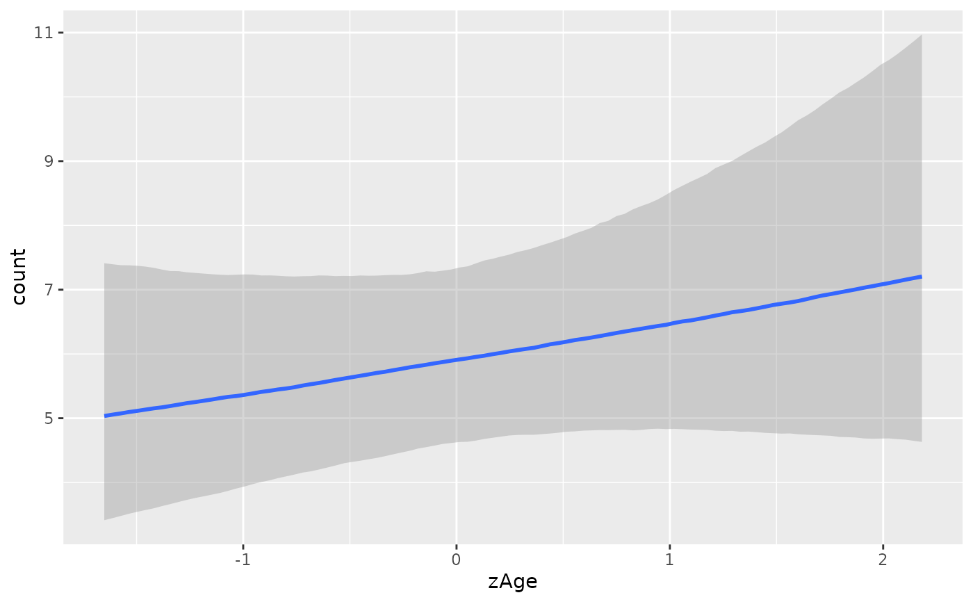
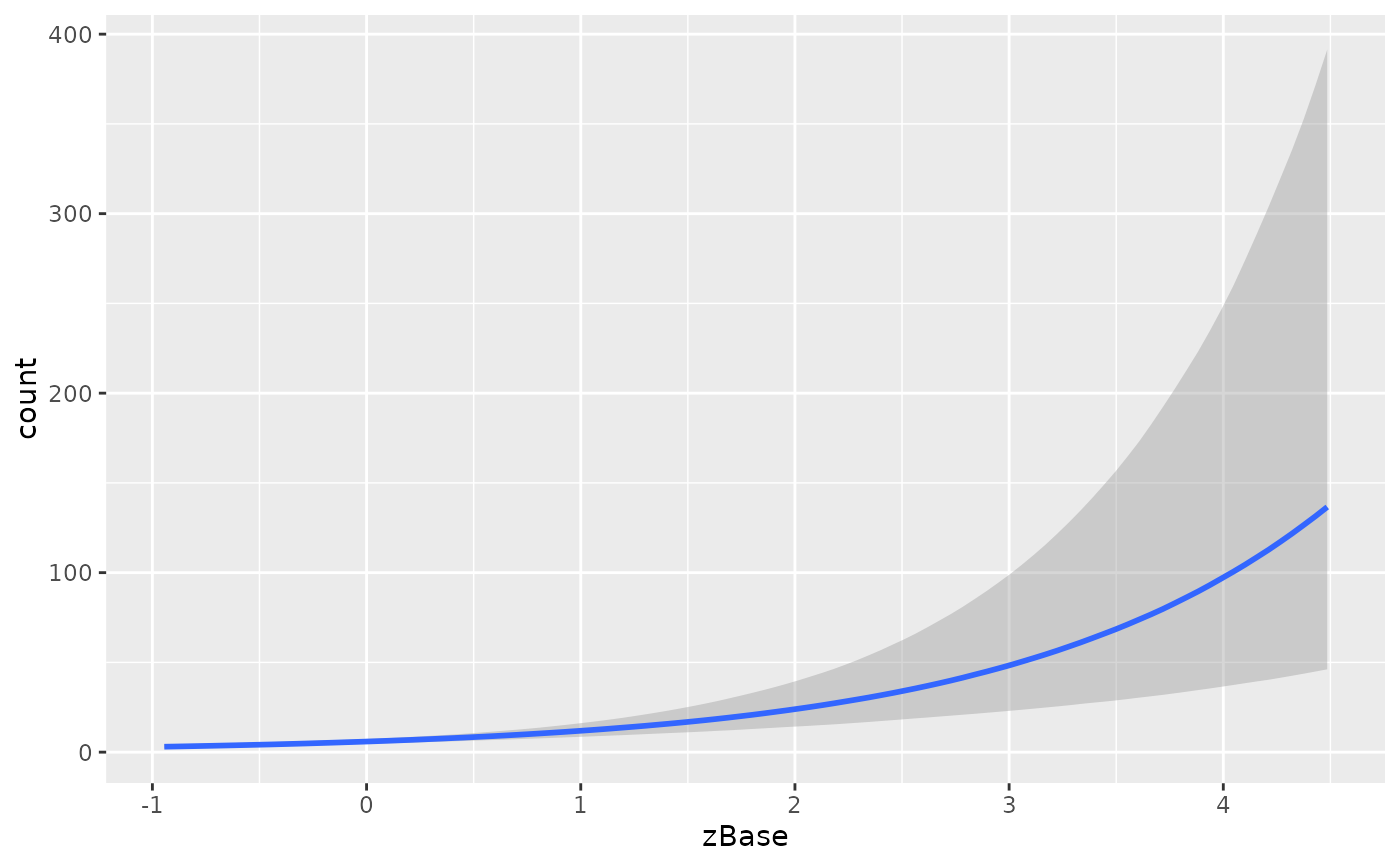
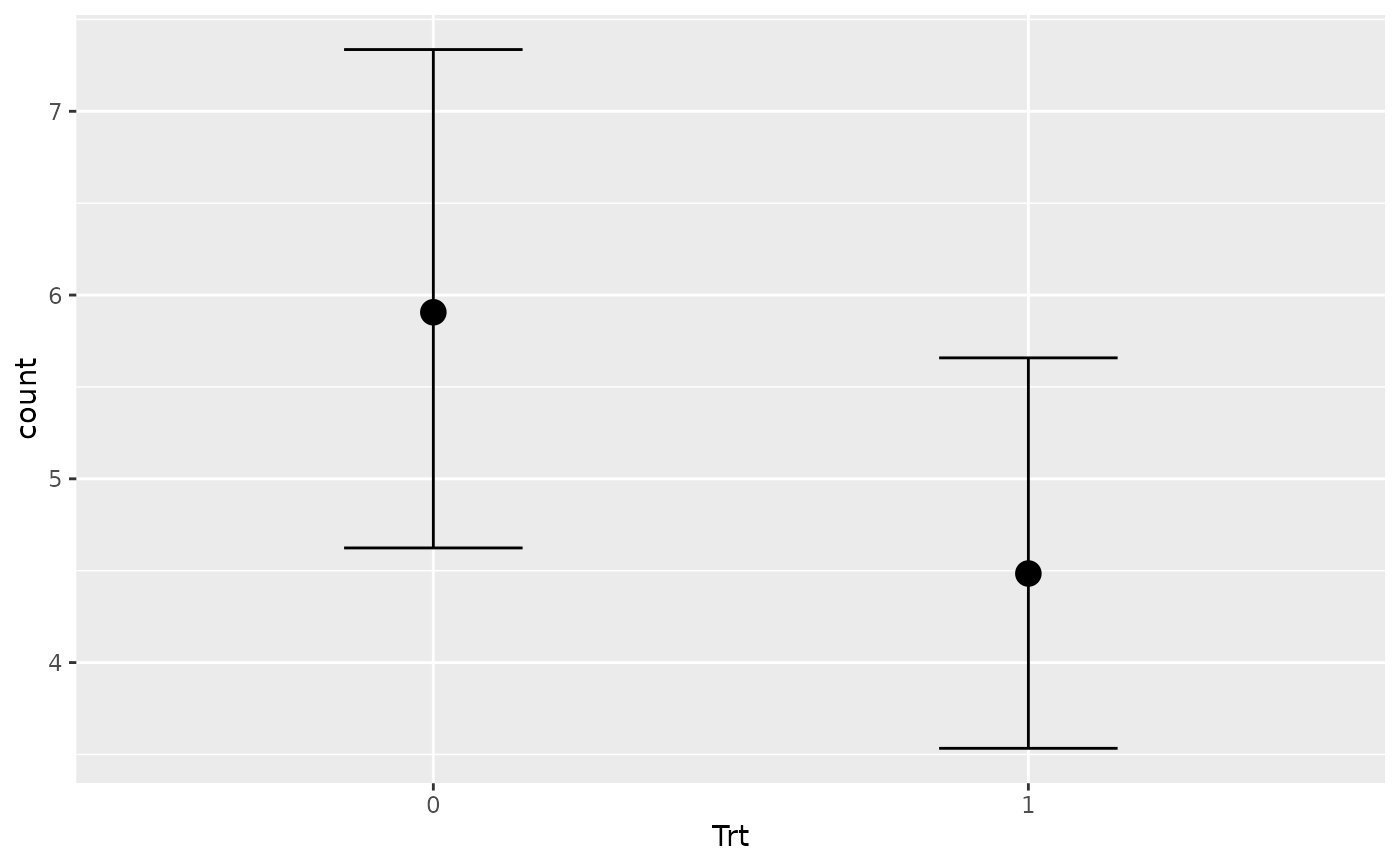
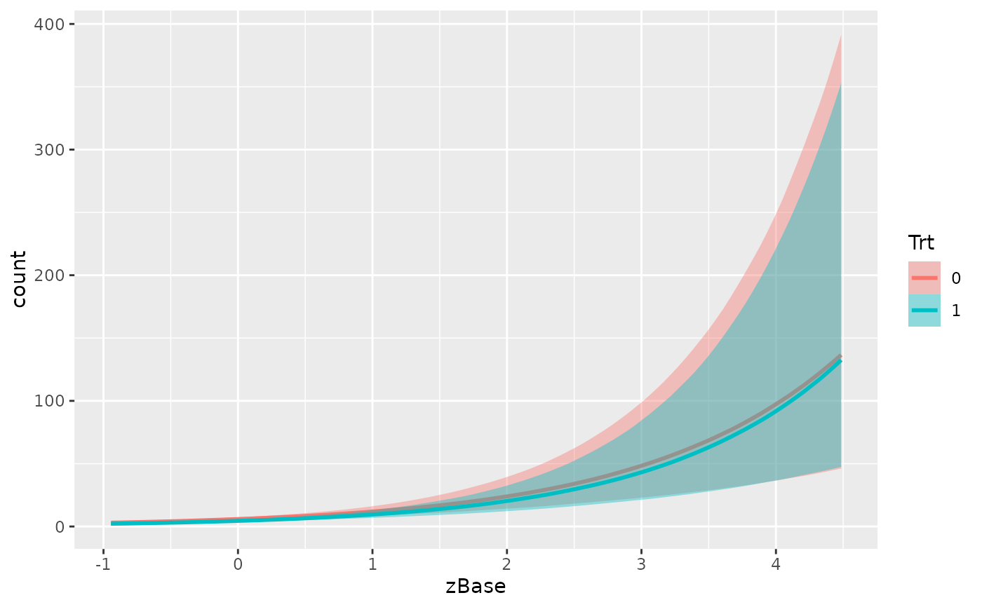
plot(conditional_effects(fit), ask = FALSE)
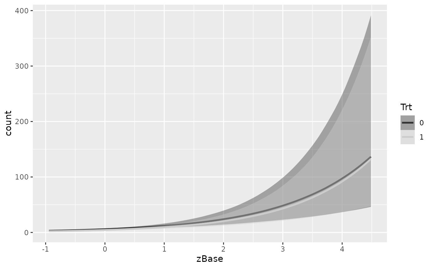
 ## change colours to grey scale
library(ggplot2)
ce <- conditional_effects(fit, "zBase:Trt")
plot(ce, plot = FALSE)[[1]] +
scale_color_grey() +
scale_fill_grey()
## change colours to grey scale
library(ggplot2)
ce <- conditional_effects(fit, "zBase:Trt")
plot(ce, plot = FALSE)[[1]] +
scale_color_grey() +
scale_fill_grey()
 ## only plot the conditional interaction effect of 'zBase:Trt'
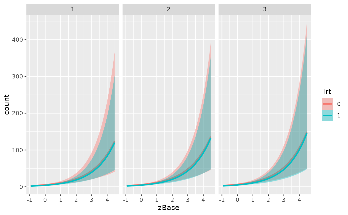
## for different values for 'zAge'
conditions <- data.frame(zAge = c(-1, 0, 1))
plot(conditional_effects(fit, effects = "zBase:Trt",
conditions = conditions))
## only plot the conditional interaction effect of 'zBase:Trt'
## for different values for 'zAge'
conditions <- data.frame(zAge = c(-1, 0, 1))
plot(conditional_effects(fit, effects = "zBase:Trt",
conditions = conditions))
 ## also incorporate group-level effects variance over patients
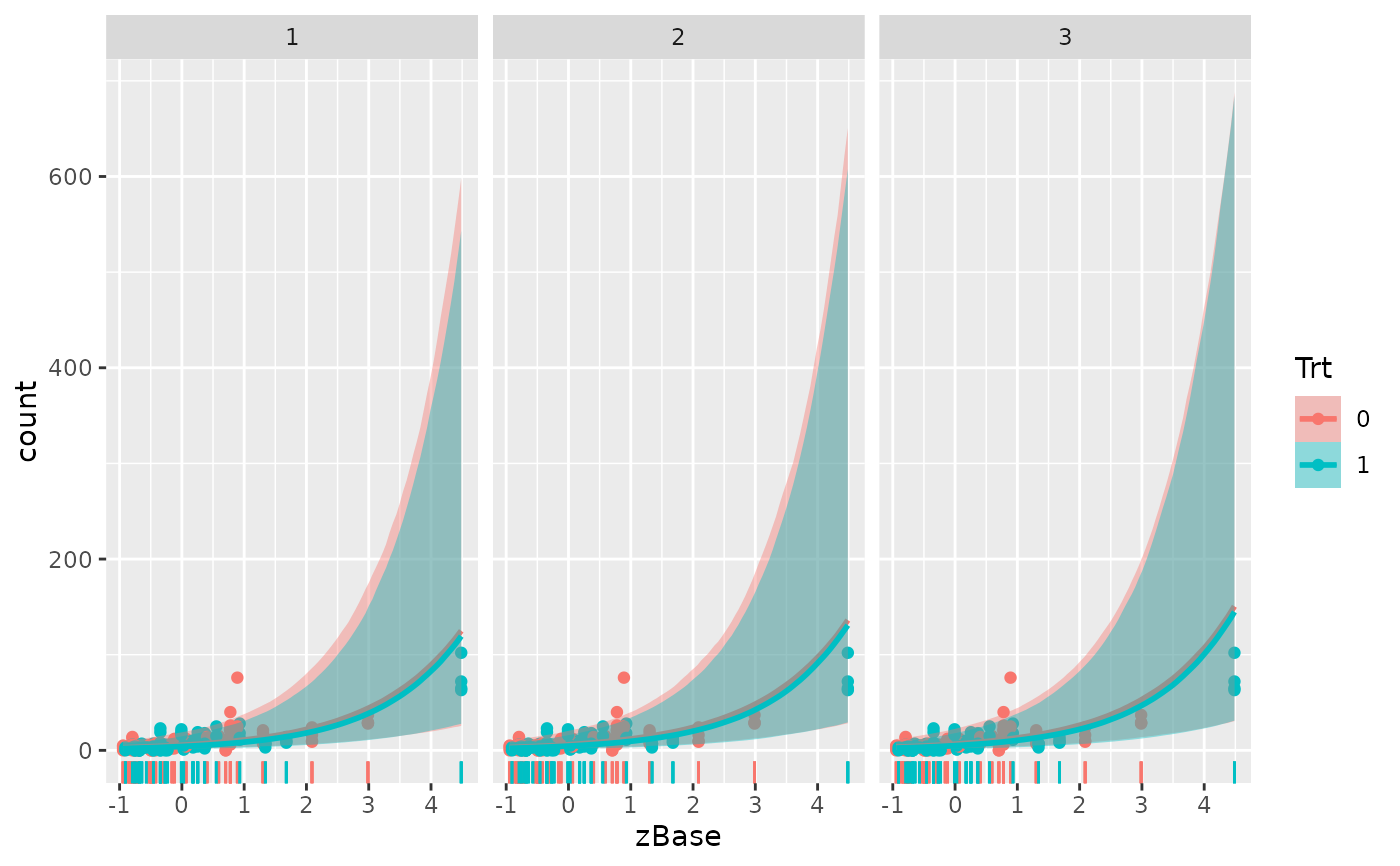
## also add data points and a rug representation of predictor values
plot(conditional_effects(fit, effects = "zBase:Trt",
conditions = conditions, re_formula = NULL),
points = TRUE, rug = TRUE)
## also incorporate group-level effects variance over patients
## also add data points and a rug representation of predictor values
plot(conditional_effects(fit, effects = "zBase:Trt",
conditions = conditions, re_formula = NULL),
points = TRUE, rug = TRUE)
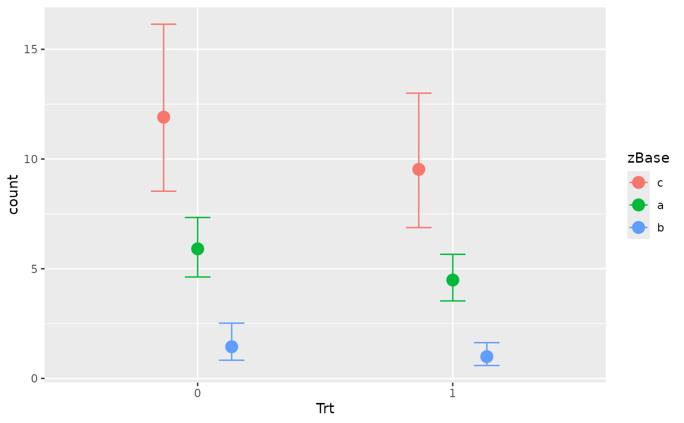
 ## change handling of two-way interactions
int_conditions <- list(
zBase = setNames(c(-2, 1, 0), c("b", "c", "a"))
)
conditional_effects(fit, effects = "Trt:zBase",
int_conditions = int_conditions)
## change handling of two-way interactions
int_conditions <- list(
zBase = setNames(c(-2, 1, 0), c("b", "c", "a"))
)
conditional_effects(fit, effects = "Trt:zBase",
int_conditions = int_conditions)
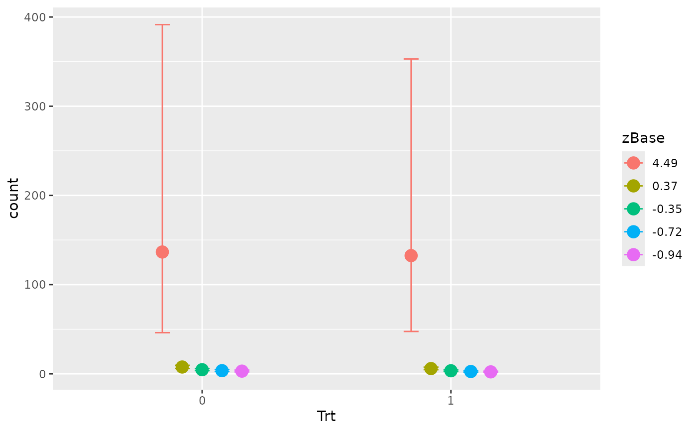
 conditional_effects(fit, effects = "Trt:zBase",
int_conditions = list(zBase = quantile))
conditional_effects(fit, effects = "Trt:zBase",
int_conditions = list(zBase = quantile))
 ## fit a model to illustrate how to plot 3-way interactions
fit3way <- brm(count ~ zAge * zBase * Trt, data = epilepsy)
#> Compiling Stan program...
#> Start sampling
#>
#> SAMPLING FOR MODEL 'anon_model' NOW (CHAIN 1).
#> Chain 1:
#> Chain 1: Gradient evaluation took 1.2e-05 seconds
#> Chain 1: 1000 transitions using 10 leapfrog steps per transition would take 0.12 seconds.
#> Chain 1: Adjust your expectations accordingly!
#> Chain 1:
#> Chain 1:
#> Chain 1: Iteration: 1 / 2000 [ 0%] (Warmup)
#> Chain 1: Iteration: 200 / 2000 [ 10%] (Warmup)
#> Chain 1: Iteration: 400 / 2000 [ 20%] (Warmup)
#> Chain 1: Iteration: 600 / 2000 [ 30%] (Warmup)
#> Chain 1: Iteration: 800 / 2000 [ 40%] (Warmup)
#> Chain 1: Iteration: 1000 / 2000 [ 50%] (Warmup)
#> Chain 1: Iteration: 1001 / 2000 [ 50%] (Sampling)
#> Chain 1: Iteration: 1200 / 2000 [ 60%] (Sampling)
#> Chain 1: Iteration: 1400 / 2000 [ 70%] (Sampling)
#> Chain 1: Iteration: 1600 / 2000 [ 80%] (Sampling)
#> Chain 1: Iteration: 1800 / 2000 [ 90%] (Sampling)
#> Chain 1: Iteration: 2000 / 2000 [100%] (Sampling)
#> Chain 1:
#> Chain 1: Elapsed Time: 0.078 seconds (Warm-up)
#> Chain 1: 0.056 seconds (Sampling)
#> Chain 1: 0.134 seconds (Total)
#> Chain 1:
#>
#> SAMPLING FOR MODEL 'anon_model' NOW (CHAIN 2).
#> Chain 2:
#> Chain 2: Gradient evaluation took 6e-06 seconds
#> Chain 2: 1000 transitions using 10 leapfrog steps per transition would take 0.06 seconds.
#> Chain 2: Adjust your expectations accordingly!
#> Chain 2:
#> Chain 2:
#> Chain 2: Iteration: 1 / 2000 [ 0%] (Warmup)
#> Chain 2: Iteration: 200 / 2000 [ 10%] (Warmup)
#> Chain 2: Iteration: 400 / 2000 [ 20%] (Warmup)
#> Chain 2: Iteration: 600 / 2000 [ 30%] (Warmup)
#> Chain 2: Iteration: 800 / 2000 [ 40%] (Warmup)
#> Chain 2: Iteration: 1000 / 2000 [ 50%] (Warmup)
#> Chain 2: Iteration: 1001 / 2000 [ 50%] (Sampling)
#> Chain 2: Iteration: 1200 / 2000 [ 60%] (Sampling)
#> Chain 2: Iteration: 1400 / 2000 [ 70%] (Sampling)
#> Chain 2: Iteration: 1600 / 2000 [ 80%] (Sampling)
#> Chain 2: Iteration: 1800 / 2000 [ 90%] (Sampling)
#> Chain 2: Iteration: 2000 / 2000 [100%] (Sampling)
#> Chain 2:
#> Chain 2: Elapsed Time: 0.071 seconds (Warm-up)
#> Chain 2: 0.049 seconds (Sampling)
#> Chain 2: 0.12 seconds (Total)
#> Chain 2:
#>
#> SAMPLING FOR MODEL 'anon_model' NOW (CHAIN 3).
#> Chain 3:
#> Chain 3: Gradient evaluation took 7e-06 seconds
#> Chain 3: 1000 transitions using 10 leapfrog steps per transition would take 0.07 seconds.
#> Chain 3: Adjust your expectations accordingly!
#> Chain 3:
#> Chain 3:
#> Chain 3: Iteration: 1 / 2000 [ 0%] (Warmup)
#> Chain 3: Iteration: 200 / 2000 [ 10%] (Warmup)
#> Chain 3: Iteration: 400 / 2000 [ 20%] (Warmup)
#> Chain 3: Iteration: 600 / 2000 [ 30%] (Warmup)
#> Chain 3: Iteration: 800 / 2000 [ 40%] (Warmup)
#> Chain 3: Iteration: 1000 / 2000 [ 50%] (Warmup)
#> Chain 3: Iteration: 1001 / 2000 [ 50%] (Sampling)
#> Chain 3: Iteration: 1200 / 2000 [ 60%] (Sampling)
#> Chain 3: Iteration: 1400 / 2000 [ 70%] (Sampling)
#> Chain 3: Iteration: 1600 / 2000 [ 80%] (Sampling)
#> Chain 3: Iteration: 1800 / 2000 [ 90%] (Sampling)
#> Chain 3: Iteration: 2000 / 2000 [100%] (Sampling)
#> Chain 3:
#> Chain 3: Elapsed Time: 0.074 seconds (Warm-up)
#> Chain 3: 0.049 seconds (Sampling)
#> Chain 3: 0.123 seconds (Total)
#> Chain 3:
#>
#> SAMPLING FOR MODEL 'anon_model' NOW (CHAIN 4).
#> Chain 4:
#> Chain 4: Gradient evaluation took 7e-06 seconds
#> Chain 4: 1000 transitions using 10 leapfrog steps per transition would take 0.07 seconds.
#> Chain 4: Adjust your expectations accordingly!
#> Chain 4:
#> Chain 4:
#> Chain 4: Iteration: 1 / 2000 [ 0%] (Warmup)
#> Chain 4: Iteration: 200 / 2000 [ 10%] (Warmup)
#> Chain 4: Iteration: 400 / 2000 [ 20%] (Warmup)
#> Chain 4: Iteration: 600 / 2000 [ 30%] (Warmup)
#> Chain 4: Iteration: 800 / 2000 [ 40%] (Warmup)
#> Chain 4: Iteration: 1000 / 2000 [ 50%] (Warmup)
#> Chain 4: Iteration: 1001 / 2000 [ 50%] (Sampling)
#> Chain 4: Iteration: 1200 / 2000 [ 60%] (Sampling)
#> Chain 4: Iteration: 1400 / 2000 [ 70%] (Sampling)
#> Chain 4: Iteration: 1600 / 2000 [ 80%] (Sampling)
#> Chain 4: Iteration: 1800 / 2000 [ 90%] (Sampling)
#> Chain 4: Iteration: 2000 / 2000 [100%] (Sampling)
#> Chain 4:
#> Chain 4: Elapsed Time: 0.071 seconds (Warm-up)
#> Chain 4: 0.05 seconds (Sampling)
#> Chain 4: 0.121 seconds (Total)
#> Chain 4:
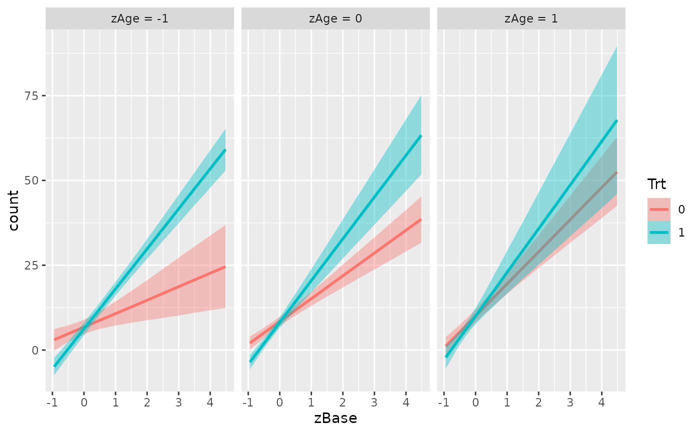
conditions <- make_conditions(fit3way, "zAge")
conditional_effects(fit3way, "zBase:Trt", conditions = conditions)
## fit a model to illustrate how to plot 3-way interactions
fit3way <- brm(count ~ zAge * zBase * Trt, data = epilepsy)
#> Compiling Stan program...
#> Start sampling
#>
#> SAMPLING FOR MODEL 'anon_model' NOW (CHAIN 1).
#> Chain 1:
#> Chain 1: Gradient evaluation took 1.2e-05 seconds
#> Chain 1: 1000 transitions using 10 leapfrog steps per transition would take 0.12 seconds.
#> Chain 1: Adjust your expectations accordingly!
#> Chain 1:
#> Chain 1:
#> Chain 1: Iteration: 1 / 2000 [ 0%] (Warmup)
#> Chain 1: Iteration: 200 / 2000 [ 10%] (Warmup)
#> Chain 1: Iteration: 400 / 2000 [ 20%] (Warmup)
#> Chain 1: Iteration: 600 / 2000 [ 30%] (Warmup)
#> Chain 1: Iteration: 800 / 2000 [ 40%] (Warmup)
#> Chain 1: Iteration: 1000 / 2000 [ 50%] (Warmup)
#> Chain 1: Iteration: 1001 / 2000 [ 50%] (Sampling)
#> Chain 1: Iteration: 1200 / 2000 [ 60%] (Sampling)
#> Chain 1: Iteration: 1400 / 2000 [ 70%] (Sampling)
#> Chain 1: Iteration: 1600 / 2000 [ 80%] (Sampling)
#> Chain 1: Iteration: 1800 / 2000 [ 90%] (Sampling)
#> Chain 1: Iteration: 2000 / 2000 [100%] (Sampling)
#> Chain 1:
#> Chain 1: Elapsed Time: 0.078 seconds (Warm-up)
#> Chain 1: 0.056 seconds (Sampling)
#> Chain 1: 0.134 seconds (Total)
#> Chain 1:
#>
#> SAMPLING FOR MODEL 'anon_model' NOW (CHAIN 2).
#> Chain 2:
#> Chain 2: Gradient evaluation took 6e-06 seconds
#> Chain 2: 1000 transitions using 10 leapfrog steps per transition would take 0.06 seconds.
#> Chain 2: Adjust your expectations accordingly!
#> Chain 2:
#> Chain 2:
#> Chain 2: Iteration: 1 / 2000 [ 0%] (Warmup)
#> Chain 2: Iteration: 200 / 2000 [ 10%] (Warmup)
#> Chain 2: Iteration: 400 / 2000 [ 20%] (Warmup)
#> Chain 2: Iteration: 600 / 2000 [ 30%] (Warmup)
#> Chain 2: Iteration: 800 / 2000 [ 40%] (Warmup)
#> Chain 2: Iteration: 1000 / 2000 [ 50%] (Warmup)
#> Chain 2: Iteration: 1001 / 2000 [ 50%] (Sampling)
#> Chain 2: Iteration: 1200 / 2000 [ 60%] (Sampling)
#> Chain 2: Iteration: 1400 / 2000 [ 70%] (Sampling)
#> Chain 2: Iteration: 1600 / 2000 [ 80%] (Sampling)
#> Chain 2: Iteration: 1800 / 2000 [ 90%] (Sampling)
#> Chain 2: Iteration: 2000 / 2000 [100%] (Sampling)
#> Chain 2:
#> Chain 2: Elapsed Time: 0.071 seconds (Warm-up)
#> Chain 2: 0.049 seconds (Sampling)
#> Chain 2: 0.12 seconds (Total)
#> Chain 2:
#>
#> SAMPLING FOR MODEL 'anon_model' NOW (CHAIN 3).
#> Chain 3:
#> Chain 3: Gradient evaluation took 7e-06 seconds
#> Chain 3: 1000 transitions using 10 leapfrog steps per transition would take 0.07 seconds.
#> Chain 3: Adjust your expectations accordingly!
#> Chain 3:
#> Chain 3:
#> Chain 3: Iteration: 1 / 2000 [ 0%] (Warmup)
#> Chain 3: Iteration: 200 / 2000 [ 10%] (Warmup)
#> Chain 3: Iteration: 400 / 2000 [ 20%] (Warmup)
#> Chain 3: Iteration: 600 / 2000 [ 30%] (Warmup)
#> Chain 3: Iteration: 800 / 2000 [ 40%] (Warmup)
#> Chain 3: Iteration: 1000 / 2000 [ 50%] (Warmup)
#> Chain 3: Iteration: 1001 / 2000 [ 50%] (Sampling)
#> Chain 3: Iteration: 1200 / 2000 [ 60%] (Sampling)
#> Chain 3: Iteration: 1400 / 2000 [ 70%] (Sampling)
#> Chain 3: Iteration: 1600 / 2000 [ 80%] (Sampling)
#> Chain 3: Iteration: 1800 / 2000 [ 90%] (Sampling)
#> Chain 3: Iteration: 2000 / 2000 [100%] (Sampling)
#> Chain 3:
#> Chain 3: Elapsed Time: 0.074 seconds (Warm-up)
#> Chain 3: 0.049 seconds (Sampling)
#> Chain 3: 0.123 seconds (Total)
#> Chain 3:
#>
#> SAMPLING FOR MODEL 'anon_model' NOW (CHAIN 4).
#> Chain 4:
#> Chain 4: Gradient evaluation took 7e-06 seconds
#> Chain 4: 1000 transitions using 10 leapfrog steps per transition would take 0.07 seconds.
#> Chain 4: Adjust your expectations accordingly!
#> Chain 4:
#> Chain 4:
#> Chain 4: Iteration: 1 / 2000 [ 0%] (Warmup)
#> Chain 4: Iteration: 200 / 2000 [ 10%] (Warmup)
#> Chain 4: Iteration: 400 / 2000 [ 20%] (Warmup)
#> Chain 4: Iteration: 600 / 2000 [ 30%] (Warmup)
#> Chain 4: Iteration: 800 / 2000 [ 40%] (Warmup)
#> Chain 4: Iteration: 1000 / 2000 [ 50%] (Warmup)
#> Chain 4: Iteration: 1001 / 2000 [ 50%] (Sampling)
#> Chain 4: Iteration: 1200 / 2000 [ 60%] (Sampling)
#> Chain 4: Iteration: 1400 / 2000 [ 70%] (Sampling)
#> Chain 4: Iteration: 1600 / 2000 [ 80%] (Sampling)
#> Chain 4: Iteration: 1800 / 2000 [ 90%] (Sampling)
#> Chain 4: Iteration: 2000 / 2000 [100%] (Sampling)
#> Chain 4:
#> Chain 4: Elapsed Time: 0.071 seconds (Warm-up)
#> Chain 4: 0.05 seconds (Sampling)
#> Chain 4: 0.121 seconds (Total)
#> Chain 4:
conditions <- make_conditions(fit3way, "zAge")
conditional_effects(fit3way, "zBase:Trt", conditions = conditions)
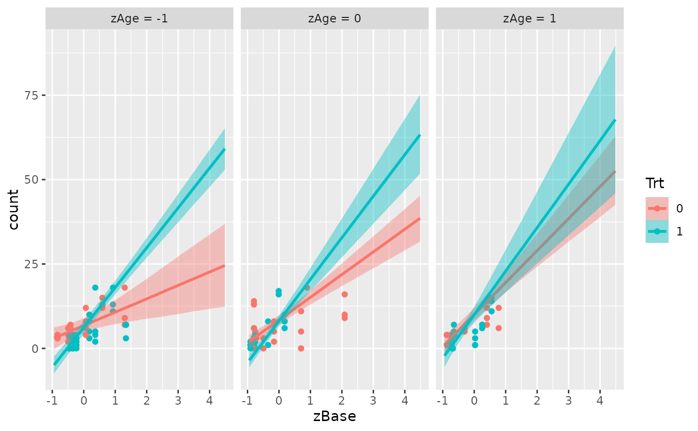
 ## only include points close to the specified values of zAge
ce <- conditional_effects(
fit3way, "zBase:Trt", conditions = conditions,
select_points = 0.1
)
plot(ce, points = TRUE)
## only include points close to the specified values of zAge
ce <- conditional_effects(
fit3way, "zBase:Trt", conditions = conditions,
select_points = 0.1
)
plot(ce, points = TRUE)
 # }
# }