
Set up a Gaussian process (GP) term in brms. The function does not evaluate its arguments – it exists purely to help set up a model with GP terms.
Usage
gp(
  ...,
  by = NA,
  k = NA,
  cov = "exp_quad",
  iso = TRUE,
  gr = TRUE,
  cmc = TRUE,
  scale = TRUE,
  c = 5/4
)
Arguments
- ...
One or more predictors for the GP.
- by
A numeric or factor variable of the same length as each predictor. In the numeric vector case, the elements multiply the values returned by the GP. In the factor variable case, a separate GP is fitted for each factor level.
- k
Optional number of basis functions for computing Hilbert-space approximate GPs. If
NA(the default), exact GPs are computed.- cov
Name of the covariance kernel. Currently supported are
"exp_quad"(exponentiated-quadratic kernel; default),"matern32"(Matern 3/2 kernel),"matern52"(Matern 5/2 kernel), and"exponential"(exponential kernel; alias:"matern12").- iso
A flag to indicate whether an isotropic (
TRUE; the default) or a non-isotropic GP should be used. In the former case, the same amount of smoothing is applied to all predictors. In the latter case, predictors may have different smoothing. Ignored if only a single predictor is supplied.- gr
Logical; Indicates if auto-grouping should be used (defaults to
TRUE). If enabled, observations sharing the same predictor values will be represented by the same latent variable in the GP. This will improve sampling efficiency drastically if the number of unique predictor combinations is small relative to the number of observations.- cmc
Logical; Only relevant if
byis a factor. IfTRUE(the default), cell-mean coding is used for theby-factor, that is one GP per level is estimated. IfFALSE, contrast GPs are estimated according to the contrasts set for theby-factor.- scale
Logical; If
TRUE(the default), predictors are scaled so that the maximum Euclidean distance between two points is 1. This often improves sampling speed and convergence. Scaling also affects the estimated length-scale parameters in that they resemble those of scaled predictors (not of the original predictors) ifscaleisTRUE.- c
Numeric value only used in approximate GPs. Defines the multiplicative constant of the predictors' range over which predictions should be computed. A good default could be
c = 5/4but we are still working on providing better recommendations.
Value
An object of class 'gp_term', which is a list
of arguments to be interpreted by the formula
parsing functions of brms.
Details
A GP is a stochastic process, which describes the relation between one or more predictors \(x = (x_1, ..., x_d)\) and a response \(f(x)\), where \(d\) is the number of predictors. A GP is the generalization of the multivariate normal distribution to an infinite number of dimensions. Thus, it can be interpreted as a prior over functions. The values of \(f( )\) at any finite set of locations are jointly multivariate normal, with a covariance matrix defined by the covariance kernel \(k_p(x_i, x_j)\), where \(p\) is the vector of parameters of the GP: $$(f(x_1), \ldots f(x_n) \sim MVN(0, (k_p(x_i, x_j))_{i,j=1}^n) .$$ The smoothness and general behavior of the function \(f\) depends only on the choice of covariance kernel. For a more detailed introduction to Gaussian processes, see https://en.wikipedia.org/wiki/Gaussian_process.
For mathematical details on the supported kernels, please see the Stan manual: https://mc-stan.org/docs/functions-reference/matrix_operations.html under "Gaussian Process Covariance Functions".
There are several parameters estimated for GPs, the most important of which are as follows:
| Parameter | Notation | Support | Meaning |
lscale | \(\ell\) | \(\mathbb{R}^+\) | length-scale of the GP's covariance kernel |
sdgp | \(\sigma\) | \(\mathbb{R}^+\) | marginal standard deviation of the GP's covariance kernel |
zgp | \(z\) | \(\mathbb{R}\) | latent variable values of the training data |
Assuming an exponentiated quadratic covariance structure, the parameters can be broadly interpreted as follows (see also https://mc-stan.org/docs/stan-users-guide/gaussian-processes.html#gaussian-process-regression). Note that in the above documentation the parameter \(\sigma\) is denoted as \(\alpha\) instead, and the parameter \(\ell\) as \(\rho\). The length-scale \(\ell\) controls the frequency of the functions represented by the GP prior i.e., values of \(\ell \gg 0\) lead to lower-frequency functions, while values of \(\ell \approx 0\) lead to higher-frequency functions. In slightly simpler terms, \(\ell\) sets the distance over which observations in the input space are strongly correlated. The marginal standard deviation \(\sigma\) controls the magnitude of the range of the function represented by the GP i.e., it represents how much the values of the function tend to deviate from the mean level. Lastly, the parameter \(z\) represents latent variable values per observation (or unique input point).
Examples
# \dontrun{
# simulate data using the mgcv package
dat <- mgcv::gamSim(1, n = 30, scale = 2)
#> Gu & Wahba 4 term additive model
# fit a simple GP model
fit1 <- brm(y ~ gp(x2), dat, chains = 2)
#> Compiling Stan program...
#> Start sampling
#>
#> SAMPLING FOR MODEL 'anon_model' NOW (CHAIN 1).
#> Chain 1:
#> Chain 1: Gradient evaluation took 5.2e-05 seconds
#> Chain 1: 1000 transitions using 10 leapfrog steps per transition would take 0.52 seconds.
#> Chain 1: Adjust your expectations accordingly!
#> Chain 1:
#> Chain 1:
#> Chain 1: Iteration: 1 / 2000 [ 0%] (Warmup)
#> Chain 1: Iteration: 200 / 2000 [ 10%] (Warmup)
#> Chain 1: Iteration: 400 / 2000 [ 20%] (Warmup)
#> Chain 1: Iteration: 600 / 2000 [ 30%] (Warmup)
#> Chain 1: Iteration: 800 / 2000 [ 40%] (Warmup)
#> Chain 1: Iteration: 1000 / 2000 [ 50%] (Warmup)
#> Chain 1: Iteration: 1001 / 2000 [ 50%] (Sampling)
#> Chain 1: Iteration: 1200 / 2000 [ 60%] (Sampling)
#> Chain 1: Iteration: 1400 / 2000 [ 70%] (Sampling)
#> Chain 1: Iteration: 1600 / 2000 [ 80%] (Sampling)
#> Chain 1: Iteration: 1800 / 2000 [ 90%] (Sampling)
#> Chain 1: Iteration: 2000 / 2000 [100%] (Sampling)
#> Chain 1:
#> Chain 1: Elapsed Time: 1.466 seconds (Warm-up)
#> Chain 1: 1.076 seconds (Sampling)
#> Chain 1: 2.542 seconds (Total)
#> Chain 1:
#>
#> SAMPLING FOR MODEL 'anon_model' NOW (CHAIN 2).
#> Chain 2:
#> Chain 2: Gradient evaluation took 3.9e-05 seconds
#> Chain 2: 1000 transitions using 10 leapfrog steps per transition would take 0.39 seconds.
#> Chain 2: Adjust your expectations accordingly!
#> Chain 2:
#> Chain 2:
#> Chain 2: Iteration: 1 / 2000 [ 0%] (Warmup)
#> Chain 2: Iteration: 200 / 2000 [ 10%] (Warmup)
#> Chain 2: Iteration: 400 / 2000 [ 20%] (Warmup)
#> Chain 2: Iteration: 600 / 2000 [ 30%] (Warmup)
#> Chain 2: Iteration: 800 / 2000 [ 40%] (Warmup)
#> Chain 2: Iteration: 1000 / 2000 [ 50%] (Warmup)
#> Chain 2: Iteration: 1001 / 2000 [ 50%] (Sampling)
#> Chain 2: Iteration: 1200 / 2000 [ 60%] (Sampling)
#> Chain 2: Iteration: 1400 / 2000 [ 70%] (Sampling)
#> Chain 2: Iteration: 1600 / 2000 [ 80%] (Sampling)
#> Chain 2: Iteration: 1800 / 2000 [ 90%] (Sampling)
#> Chain 2: Iteration: 2000 / 2000 [100%] (Sampling)
#> Chain 2:
#> Chain 2: Elapsed Time: 1.437 seconds (Warm-up)
#> Chain 2: 1.1 seconds (Sampling)
#> Chain 2: 2.537 seconds (Total)
#> Chain 2:
#> Warning: There were 3 divergent transitions after warmup. See
#> https://mc-stan.org/misc/warnings.html#divergent-transitions-after-warmup
#> to find out why this is a problem and how to eliminate them.
#> Warning: Examine the pairs() plot to diagnose sampling problems
#> Warning: Bulk Effective Samples Size (ESS) is too low, indicating posterior means and medians may be unreliable.
#> Running the chains for more iterations may help. See
#> https://mc-stan.org/misc/warnings.html#bulk-ess
#> Warning: Tail Effective Samples Size (ESS) is too low, indicating posterior variances and tail quantiles may be unreliable.
#> Running the chains for more iterations may help. See
#> https://mc-stan.org/misc/warnings.html#tail-ess
summary(fit1)
#> Warning: There were 3 divergent transitions after warmup. Increasing adapt_delta above 0.8 may help. See http://mc-stan.org/misc/warnings.html#divergent-transitions-after-warmup
#> Family: gaussian
#> Links: mu = identity
#> Formula: y ~ gp(x2)
#> Data: dat (Number of observations: 30)
#> Draws: 2 chains, each with iter = 2000; warmup = 1000; thin = 1;
#> total post-warmup draws = 2000
#>
#> Gaussian Process Hyperparameters:
#> Estimate Est.Error l-95% CI u-95% CI Rhat Bulk_ESS Tail_ESS
#> sdgp(gpx2) 3.67 1.87 1.09 7.52 1.01 273 409
#> lscale(gpx2) 0.12 0.10 0.03 0.31 1.01 161 215
#>
#> Regression Coefficients:
#> Estimate Est.Error l-95% CI u-95% CI Rhat Bulk_ESS Tail_ESS
#> Intercept 7.39 1.60 3.78 10.36 1.00 743 688
#>
#> Further Distributional Parameters:
#> Estimate Est.Error l-95% CI u-95% CI Rhat Bulk_ESS Tail_ESS
#> sigma 2.69 0.51 1.95 3.89 1.01 400 779
#>
#> Draws were sampled using sampling(NUTS). For each parameter, Bulk_ESS
#> and Tail_ESS are effective sample size measures, and Rhat is the potential
#> scale reduction factor on split chains (at convergence, Rhat = 1).
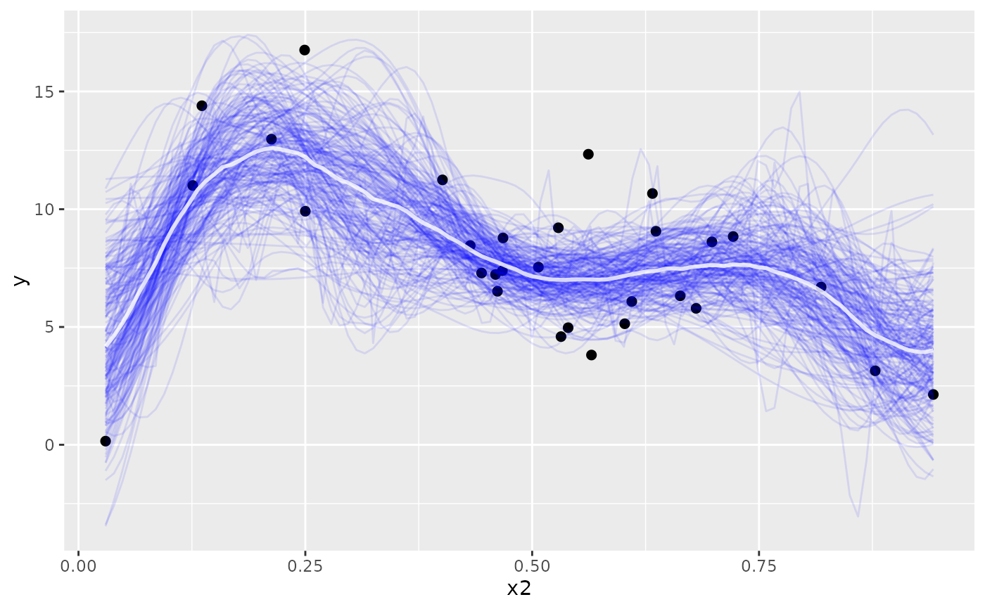
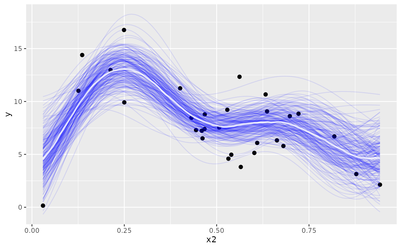
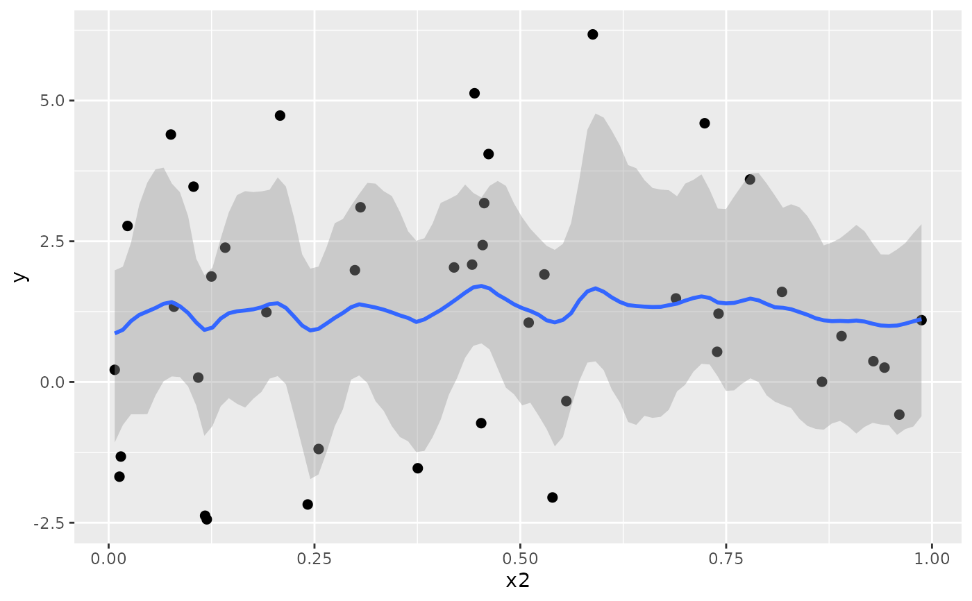
me1 <- conditional_effects(fit1, ndraws = 200, spaghetti = TRUE)
plot(me1, ask = FALSE, points = TRUE)
 # fit a more complicated GP model and use an approximate GP for x2
fit2 <- brm(y ~ gp(x0) + x1 + gp(x2, k = 10) + x3, dat, chains = 2)
#> Compiling Stan program...
#> Start sampling
#>
#> SAMPLING FOR MODEL 'anon_model' NOW (CHAIN 1).
#> Chain 1:
#> Chain 1: Gradient evaluation took 5.7e-05 seconds
#> Chain 1: 1000 transitions using 10 leapfrog steps per transition would take 0.57 seconds.
#> Chain 1: Adjust your expectations accordingly!
#> Chain 1:
#> Chain 1:
#> Chain 1: Iteration: 1 / 2000 [ 0%] (Warmup)
#> Chain 1: Iteration: 200 / 2000 [ 10%] (Warmup)
#> Chain 1: Iteration: 400 / 2000 [ 20%] (Warmup)
#> Chain 1: Iteration: 600 / 2000 [ 30%] (Warmup)
#> Chain 1: Iteration: 800 / 2000 [ 40%] (Warmup)
#> Chain 1: Iteration: 1000 / 2000 [ 50%] (Warmup)
#> Chain 1: Iteration: 1001 / 2000 [ 50%] (Sampling)
#> Chain 1: Iteration: 1200 / 2000 [ 60%] (Sampling)
#> Chain 1: Iteration: 1400 / 2000 [ 70%] (Sampling)
#> Chain 1: Iteration: 1600 / 2000 [ 80%] (Sampling)
#> Chain 1: Iteration: 1800 / 2000 [ 90%] (Sampling)
#> Chain 1: Iteration: 2000 / 2000 [100%] (Sampling)
#> Chain 1:
#> Chain 1: Elapsed Time: 1.714 seconds (Warm-up)
#> Chain 1: 1.512 seconds (Sampling)
#> Chain 1: 3.226 seconds (Total)
#> Chain 1:
#>
#> SAMPLING FOR MODEL 'anon_model' NOW (CHAIN 2).
#> Chain 2:
#> Chain 2: Gradient evaluation took 5.4e-05 seconds
#> Chain 2: 1000 transitions using 10 leapfrog steps per transition would take 0.54 seconds.
#> Chain 2: Adjust your expectations accordingly!
#> Chain 2:
#> Chain 2:
#> Chain 2: Iteration: 1 / 2000 [ 0%] (Warmup)
#> Chain 2: Iteration: 200 / 2000 [ 10%] (Warmup)
#> Chain 2: Iteration: 400 / 2000 [ 20%] (Warmup)
#> Chain 2: Iteration: 600 / 2000 [ 30%] (Warmup)
#> Chain 2: Iteration: 800 / 2000 [ 40%] (Warmup)
#> Chain 2: Iteration: 1000 / 2000 [ 50%] (Warmup)
#> Chain 2: Iteration: 1001 / 2000 [ 50%] (Sampling)
#> Chain 2: Iteration: 1200 / 2000 [ 60%] (Sampling)
#> Chain 2: Iteration: 1400 / 2000 [ 70%] (Sampling)
#> Chain 2: Iteration: 1600 / 2000 [ 80%] (Sampling)
#> Chain 2: Iteration: 1800 / 2000 [ 90%] (Sampling)
#> Chain 2: Iteration: 2000 / 2000 [100%] (Sampling)
#> Chain 2:
#> Chain 2: Elapsed Time: 1.672 seconds (Warm-up)
#> Chain 2: 1.241 seconds (Sampling)
#> Chain 2: 2.913 seconds (Total)
#> Chain 2:
#> Warning: There were 12 divergent transitions after warmup. See
#> https://mc-stan.org/misc/warnings.html#divergent-transitions-after-warmup
#> to find out why this is a problem and how to eliminate them.
#> Warning: Examine the pairs() plot to diagnose sampling problems
summary(fit2)
#> Warning: There were 12 divergent transitions after warmup. Increasing adapt_delta above 0.8 may help. See http://mc-stan.org/misc/warnings.html#divergent-transitions-after-warmup
#> Family: gaussian
#> Links: mu = identity
#> Formula: y ~ gp(x0) + x1 + gp(x2, k = 10) + x3
#> Data: dat (Number of observations: 30)
#> Draws: 2 chains, each with iter = 2000; warmup = 1000; thin = 1;
#> total post-warmup draws = 2000
#>
#> Gaussian Process Hyperparameters:
#> Estimate Est.Error l-95% CI u-95% CI Rhat Bulk_ESS Tail_ESS
#> sdgp(gpx0) 0.78 0.69 0.03 2.54 1.00 829 771
#> sdgp(gpx2) 5.41 2.39 2.17 10.90 1.00 588 630
#> lscale(gpx0) 0.13 0.28 0.01 0.78 1.00 631 564
#> lscale(gpx2) 0.06 0.05 0.01 0.19 1.01 1057 1388
#>
#> Regression Coefficients:
#> Estimate Est.Error l-95% CI u-95% CI Rhat Bulk_ESS Tail_ESS
#> Intercept 4.55 1.83 0.87 8.09 1.00 1211 1285
#> x1 4.83 1.54 1.91 7.94 1.00 1556 1193
#> x3 0.91 1.51 -1.99 3.85 1.00 1892 1424
#>
#> Further Distributional Parameters:
#> Estimate Est.Error l-95% CI u-95% CI Rhat Bulk_ESS Tail_ESS
#> sigma 2.16 0.39 1.53 3.07 1.00 876 577
#>
#> Draws were sampled using sampling(NUTS). For each parameter, Bulk_ESS
#> and Tail_ESS are effective sample size measures, and Rhat is the potential
#> scale reduction factor on split chains (at convergence, Rhat = 1).
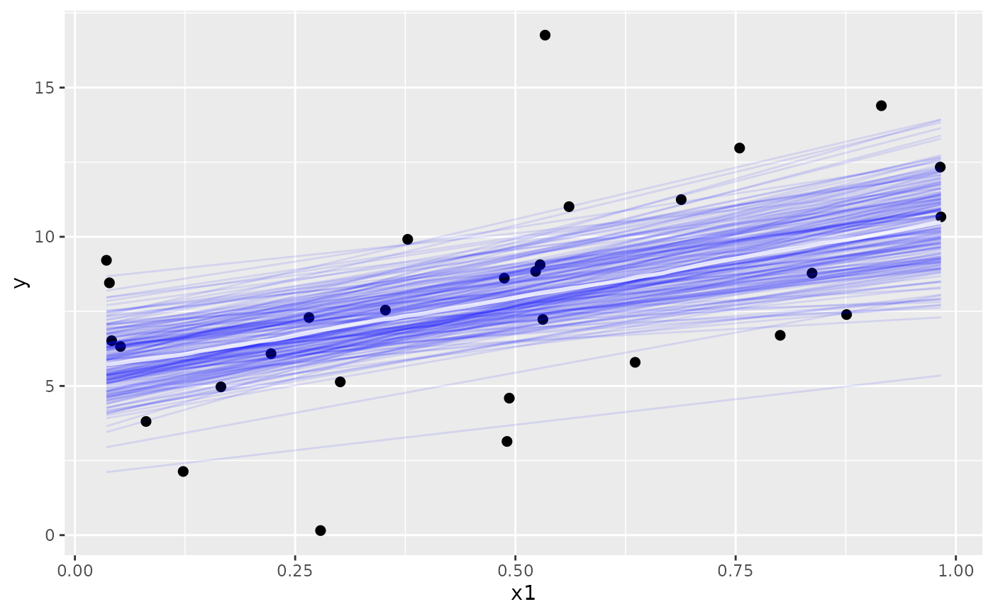
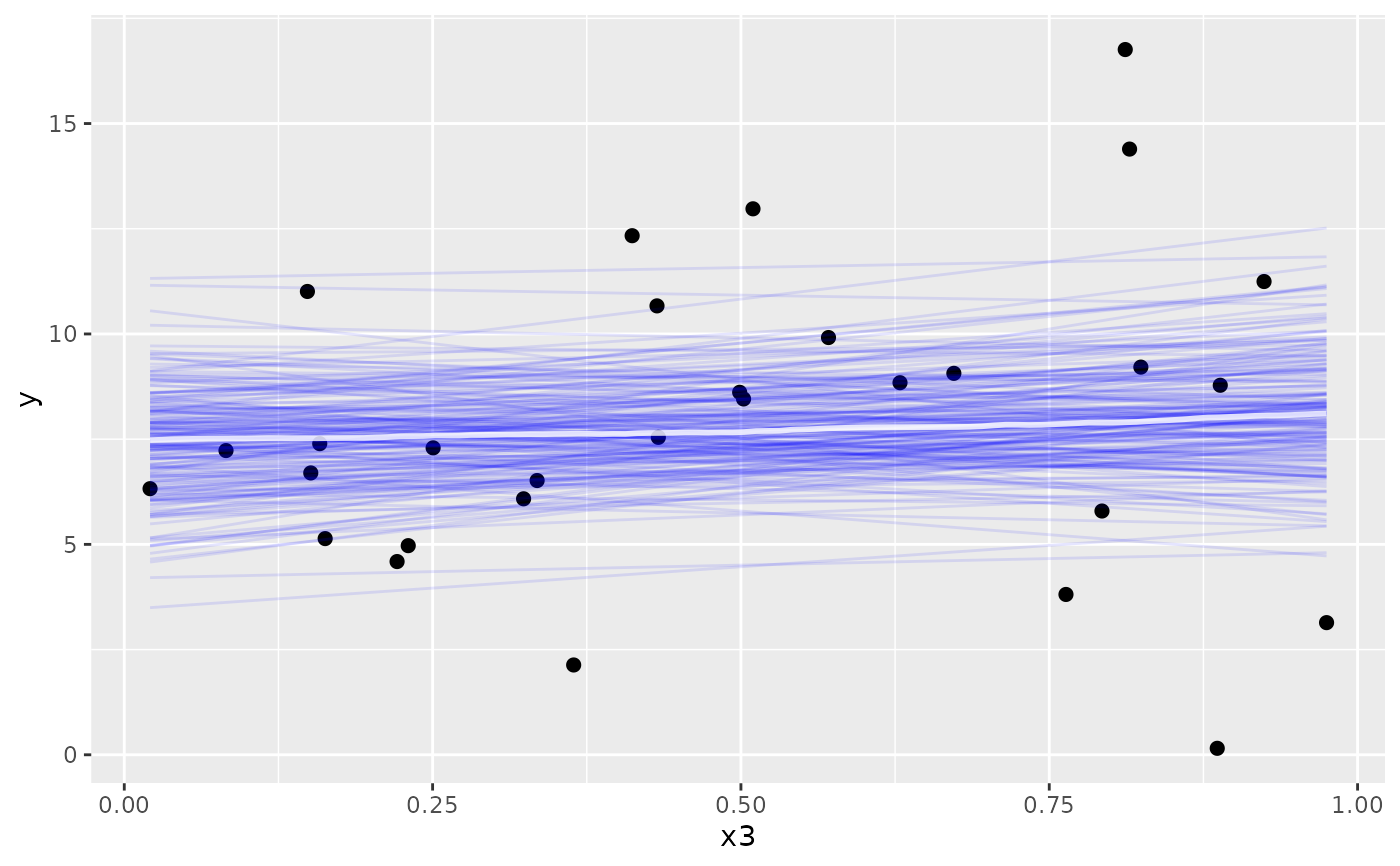
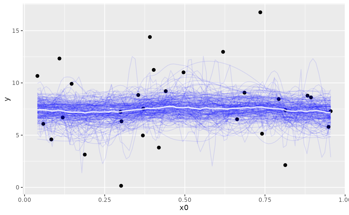
me2 <- conditional_effects(fit2, ndraws = 200, spaghetti = TRUE)
plot(me2, ask = FALSE, points = TRUE)
# fit a more complicated GP model and use an approximate GP for x2
fit2 <- brm(y ~ gp(x0) + x1 + gp(x2, k = 10) + x3, dat, chains = 2)
#> Compiling Stan program...
#> Start sampling
#>
#> SAMPLING FOR MODEL 'anon_model' NOW (CHAIN 1).
#> Chain 1:
#> Chain 1: Gradient evaluation took 5.7e-05 seconds
#> Chain 1: 1000 transitions using 10 leapfrog steps per transition would take 0.57 seconds.
#> Chain 1: Adjust your expectations accordingly!
#> Chain 1:
#> Chain 1:
#> Chain 1: Iteration: 1 / 2000 [ 0%] (Warmup)
#> Chain 1: Iteration: 200 / 2000 [ 10%] (Warmup)
#> Chain 1: Iteration: 400 / 2000 [ 20%] (Warmup)
#> Chain 1: Iteration: 600 / 2000 [ 30%] (Warmup)
#> Chain 1: Iteration: 800 / 2000 [ 40%] (Warmup)
#> Chain 1: Iteration: 1000 / 2000 [ 50%] (Warmup)
#> Chain 1: Iteration: 1001 / 2000 [ 50%] (Sampling)
#> Chain 1: Iteration: 1200 / 2000 [ 60%] (Sampling)
#> Chain 1: Iteration: 1400 / 2000 [ 70%] (Sampling)
#> Chain 1: Iteration: 1600 / 2000 [ 80%] (Sampling)
#> Chain 1: Iteration: 1800 / 2000 [ 90%] (Sampling)
#> Chain 1: Iteration: 2000 / 2000 [100%] (Sampling)
#> Chain 1:
#> Chain 1: Elapsed Time: 1.714 seconds (Warm-up)
#> Chain 1: 1.512 seconds (Sampling)
#> Chain 1: 3.226 seconds (Total)
#> Chain 1:
#>
#> SAMPLING FOR MODEL 'anon_model' NOW (CHAIN 2).
#> Chain 2:
#> Chain 2: Gradient evaluation took 5.4e-05 seconds
#> Chain 2: 1000 transitions using 10 leapfrog steps per transition would take 0.54 seconds.
#> Chain 2: Adjust your expectations accordingly!
#> Chain 2:
#> Chain 2:
#> Chain 2: Iteration: 1 / 2000 [ 0%] (Warmup)
#> Chain 2: Iteration: 200 / 2000 [ 10%] (Warmup)
#> Chain 2: Iteration: 400 / 2000 [ 20%] (Warmup)
#> Chain 2: Iteration: 600 / 2000 [ 30%] (Warmup)
#> Chain 2: Iteration: 800 / 2000 [ 40%] (Warmup)
#> Chain 2: Iteration: 1000 / 2000 [ 50%] (Warmup)
#> Chain 2: Iteration: 1001 / 2000 [ 50%] (Sampling)
#> Chain 2: Iteration: 1200 / 2000 [ 60%] (Sampling)
#> Chain 2: Iteration: 1400 / 2000 [ 70%] (Sampling)
#> Chain 2: Iteration: 1600 / 2000 [ 80%] (Sampling)
#> Chain 2: Iteration: 1800 / 2000 [ 90%] (Sampling)
#> Chain 2: Iteration: 2000 / 2000 [100%] (Sampling)
#> Chain 2:
#> Chain 2: Elapsed Time: 1.672 seconds (Warm-up)
#> Chain 2: 1.241 seconds (Sampling)
#> Chain 2: 2.913 seconds (Total)
#> Chain 2:
#> Warning: There were 12 divergent transitions after warmup. See
#> https://mc-stan.org/misc/warnings.html#divergent-transitions-after-warmup
#> to find out why this is a problem and how to eliminate them.
#> Warning: Examine the pairs() plot to diagnose sampling problems
summary(fit2)
#> Warning: There were 12 divergent transitions after warmup. Increasing adapt_delta above 0.8 may help. See http://mc-stan.org/misc/warnings.html#divergent-transitions-after-warmup
#> Family: gaussian
#> Links: mu = identity
#> Formula: y ~ gp(x0) + x1 + gp(x2, k = 10) + x3
#> Data: dat (Number of observations: 30)
#> Draws: 2 chains, each with iter = 2000; warmup = 1000; thin = 1;
#> total post-warmup draws = 2000
#>
#> Gaussian Process Hyperparameters:
#> Estimate Est.Error l-95% CI u-95% CI Rhat Bulk_ESS Tail_ESS
#> sdgp(gpx0) 0.78 0.69 0.03 2.54 1.00 829 771
#> sdgp(gpx2) 5.41 2.39 2.17 10.90 1.00 588 630
#> lscale(gpx0) 0.13 0.28 0.01 0.78 1.00 631 564
#> lscale(gpx2) 0.06 0.05 0.01 0.19 1.01 1057 1388
#>
#> Regression Coefficients:
#> Estimate Est.Error l-95% CI u-95% CI Rhat Bulk_ESS Tail_ESS
#> Intercept 4.55 1.83 0.87 8.09 1.00 1211 1285
#> x1 4.83 1.54 1.91 7.94 1.00 1556 1193
#> x3 0.91 1.51 -1.99 3.85 1.00 1892 1424
#>
#> Further Distributional Parameters:
#> Estimate Est.Error l-95% CI u-95% CI Rhat Bulk_ESS Tail_ESS
#> sigma 2.16 0.39 1.53 3.07 1.00 876 577
#>
#> Draws were sampled using sampling(NUTS). For each parameter, Bulk_ESS
#> and Tail_ESS are effective sample size measures, and Rhat is the potential
#> scale reduction factor on split chains (at convergence, Rhat = 1).
me2 <- conditional_effects(fit2, ndraws = 200, spaghetti = TRUE)
plot(me2, ask = FALSE, points = TRUE)
 # fit a multivariate GP model with Matern 3/2 kernel
fit3 <- brm(y ~ gp(x1, x2, cov = "matern32"), dat, chains = 2)
#> Compiling Stan program...
#> Start sampling
#>
#> SAMPLING FOR MODEL 'anon_model' NOW (CHAIN 1).
#> Chain 1:
#> Chain 1: Gradient evaluation took 0.000116 seconds
#> Chain 1: 1000 transitions using 10 leapfrog steps per transition would take 1.16 seconds.
#> Chain 1: Adjust your expectations accordingly!
#> Chain 1:
#> Chain 1:
#> Chain 1: Iteration: 1 / 2000 [ 0%] (Warmup)
#> Chain 1: Iteration: 200 / 2000 [ 10%] (Warmup)
#> Chain 1: Iteration: 400 / 2000 [ 20%] (Warmup)
#> Chain 1: Iteration: 600 / 2000 [ 30%] (Warmup)
#> Chain 1: Iteration: 800 / 2000 [ 40%] (Warmup)
#> Chain 1: Iteration: 1000 / 2000 [ 50%] (Warmup)
#> Chain 1: Iteration: 1001 / 2000 [ 50%] (Sampling)
#> Chain 1: Iteration: 1200 / 2000 [ 60%] (Sampling)
#> Chain 1: Iteration: 1400 / 2000 [ 70%] (Sampling)
#> Chain 1: Iteration: 1600 / 2000 [ 80%] (Sampling)
#> Chain 1: Iteration: 1800 / 2000 [ 90%] (Sampling)
#> Chain 1: Iteration: 2000 / 2000 [100%] (Sampling)
#> Chain 1:
#> Chain 1: Elapsed Time: 4.027 seconds (Warm-up)
#> Chain 1: 3.145 seconds (Sampling)
#> Chain 1: 7.172 seconds (Total)
#> Chain 1:
#>
#> SAMPLING FOR MODEL 'anon_model' NOW (CHAIN 2).
#> Chain 2:
#> Chain 2: Gradient evaluation took 0.000138 seconds
#> Chain 2: 1000 transitions using 10 leapfrog steps per transition would take 1.38 seconds.
#> Chain 2: Adjust your expectations accordingly!
#> Chain 2:
#> Chain 2:
#> Chain 2: Iteration: 1 / 2000 [ 0%] (Warmup)
#> Chain 2: Iteration: 200 / 2000 [ 10%] (Warmup)
#> Chain 2: Iteration: 400 / 2000 [ 20%] (Warmup)
#> Chain 2: Iteration: 600 / 2000 [ 30%] (Warmup)
#> Chain 2: Iteration: 800 / 2000 [ 40%] (Warmup)
#> Chain 2: Iteration: 1000 / 2000 [ 50%] (Warmup)
#> Chain 2: Iteration: 1001 / 2000 [ 50%] (Sampling)
#> Chain 2: Iteration: 1200 / 2000 [ 60%] (Sampling)
#> Chain 2: Iteration: 1400 / 2000 [ 70%] (Sampling)
#> Chain 2: Iteration: 1600 / 2000 [ 80%] (Sampling)
#> Chain 2: Iteration: 1800 / 2000 [ 90%] (Sampling)
#> Chain 2: Iteration: 2000 / 2000 [100%] (Sampling)
#> Chain 2:
#> Chain 2: Elapsed Time: 3.672 seconds (Warm-up)
#> Chain 2: 3.405 seconds (Sampling)
#> Chain 2: 7.077 seconds (Total)
#> Chain 2:
#> Warning: There were 27 divergent transitions after warmup. See
#> https://mc-stan.org/misc/warnings.html#divergent-transitions-after-warmup
#> to find out why this is a problem and how to eliminate them.
#> Warning: Examine the pairs() plot to diagnose sampling problems
#> Warning: Bulk Effective Samples Size (ESS) is too low, indicating posterior means and medians may be unreliable.
#> Running the chains for more iterations may help. See
#> https://mc-stan.org/misc/warnings.html#bulk-ess
#> Warning: Tail Effective Samples Size (ESS) is too low, indicating posterior variances and tail quantiles may be unreliable.
#> Running the chains for more iterations may help. See
#> https://mc-stan.org/misc/warnings.html#tail-ess
summary(fit3)
#> Warning: There were 27 divergent transitions after warmup. Increasing adapt_delta above 0.8 may help. See http://mc-stan.org/misc/warnings.html#divergent-transitions-after-warmup
#> Family: gaussian
#> Links: mu = identity
#> Formula: y ~ gp(x1, x2, cov = "matern32")
#> Data: dat (Number of observations: 30)
#> Draws: 2 chains, each with iter = 2000; warmup = 1000; thin = 1;
#> total post-warmup draws = 2000
#>
#> Gaussian Process Hyperparameters:
#> Estimate Est.Error l-95% CI u-95% CI Rhat Bulk_ESS Tail_ESS
#> sdgp(gpx1x2) 3.85 1.16 1.86 6.79 1.00 234 365
#> lscale(gpx1x2) 0.21 0.13 0.08 0.55 1.01 324 546
#>
#> Regression Coefficients:
#> Estimate Est.Error l-95% CI u-95% CI Rhat Bulk_ESS Tail_ESS
#> Intercept 7.40 1.53 4.09 10.23 1.00 503 219
#>
#> Further Distributional Parameters:
#> Estimate Est.Error l-95% CI u-95% CI Rhat Bulk_ESS Tail_ESS
#> sigma 1.77 0.66 0.69 3.21 1.01 76 189
#>
#> Draws were sampled using sampling(NUTS). For each parameter, Bulk_ESS
#> and Tail_ESS are effective sample size measures, and Rhat is the potential
#> scale reduction factor on split chains (at convergence, Rhat = 1).
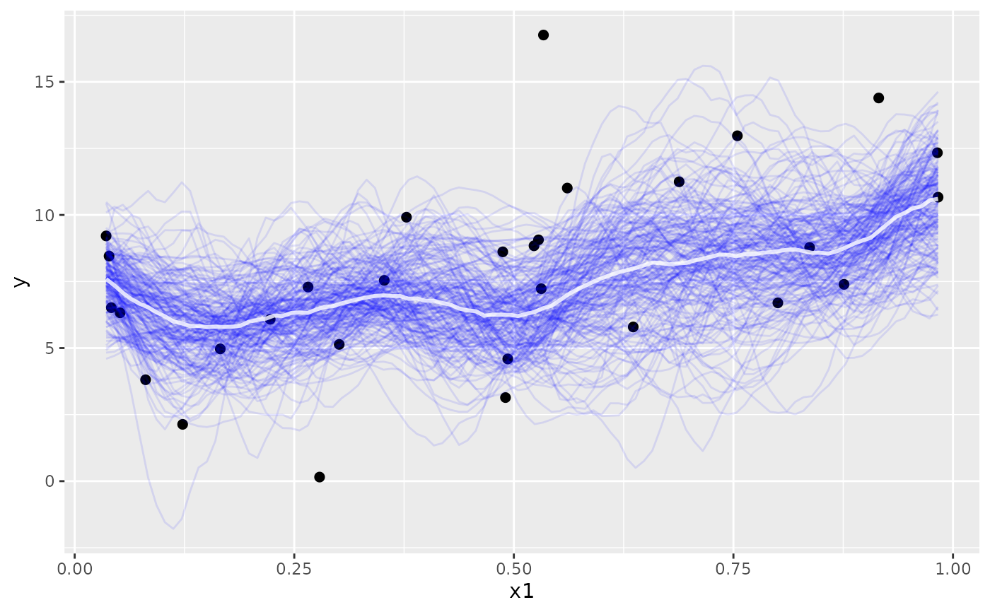
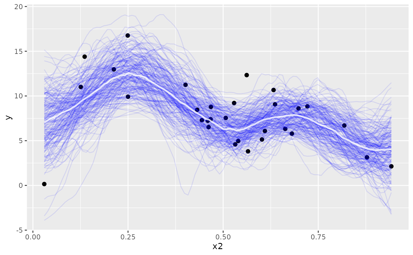
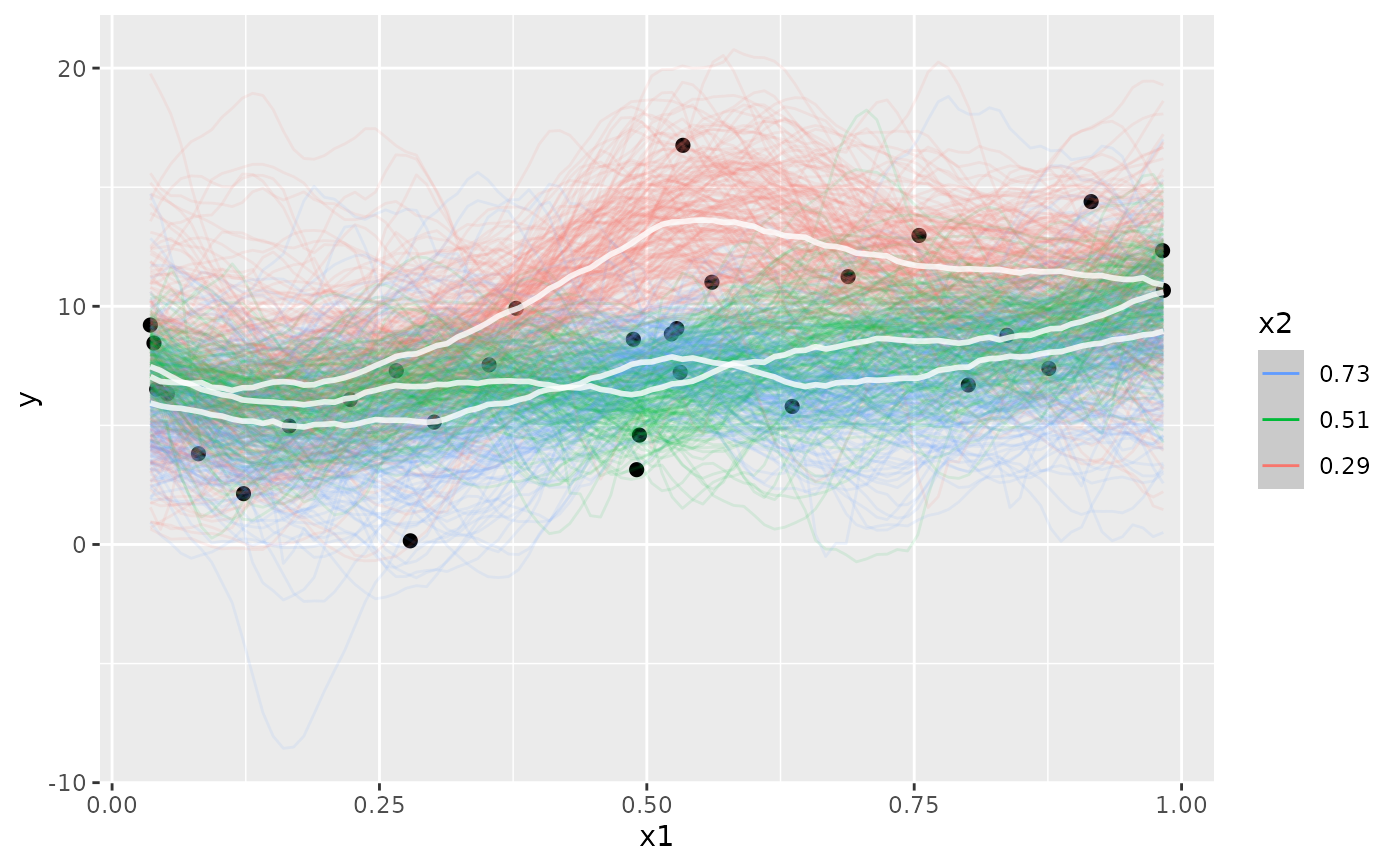
me3 <- conditional_effects(fit3, ndraws = 200, spaghetti = TRUE)
plot(me3, ask = FALSE, points = TRUE)
# fit a multivariate GP model with Matern 3/2 kernel
fit3 <- brm(y ~ gp(x1, x2, cov = "matern32"), dat, chains = 2)
#> Compiling Stan program...
#> Start sampling
#>
#> SAMPLING FOR MODEL 'anon_model' NOW (CHAIN 1).
#> Chain 1:
#> Chain 1: Gradient evaluation took 0.000116 seconds
#> Chain 1: 1000 transitions using 10 leapfrog steps per transition would take 1.16 seconds.
#> Chain 1: Adjust your expectations accordingly!
#> Chain 1:
#> Chain 1:
#> Chain 1: Iteration: 1 / 2000 [ 0%] (Warmup)
#> Chain 1: Iteration: 200 / 2000 [ 10%] (Warmup)
#> Chain 1: Iteration: 400 / 2000 [ 20%] (Warmup)
#> Chain 1: Iteration: 600 / 2000 [ 30%] (Warmup)
#> Chain 1: Iteration: 800 / 2000 [ 40%] (Warmup)
#> Chain 1: Iteration: 1000 / 2000 [ 50%] (Warmup)
#> Chain 1: Iteration: 1001 / 2000 [ 50%] (Sampling)
#> Chain 1: Iteration: 1200 / 2000 [ 60%] (Sampling)
#> Chain 1: Iteration: 1400 / 2000 [ 70%] (Sampling)
#> Chain 1: Iteration: 1600 / 2000 [ 80%] (Sampling)
#> Chain 1: Iteration: 1800 / 2000 [ 90%] (Sampling)
#> Chain 1: Iteration: 2000 / 2000 [100%] (Sampling)
#> Chain 1:
#> Chain 1: Elapsed Time: 4.027 seconds (Warm-up)
#> Chain 1: 3.145 seconds (Sampling)
#> Chain 1: 7.172 seconds (Total)
#> Chain 1:
#>
#> SAMPLING FOR MODEL 'anon_model' NOW (CHAIN 2).
#> Chain 2:
#> Chain 2: Gradient evaluation took 0.000138 seconds
#> Chain 2: 1000 transitions using 10 leapfrog steps per transition would take 1.38 seconds.
#> Chain 2: Adjust your expectations accordingly!
#> Chain 2:
#> Chain 2:
#> Chain 2: Iteration: 1 / 2000 [ 0%] (Warmup)
#> Chain 2: Iteration: 200 / 2000 [ 10%] (Warmup)
#> Chain 2: Iteration: 400 / 2000 [ 20%] (Warmup)
#> Chain 2: Iteration: 600 / 2000 [ 30%] (Warmup)
#> Chain 2: Iteration: 800 / 2000 [ 40%] (Warmup)
#> Chain 2: Iteration: 1000 / 2000 [ 50%] (Warmup)
#> Chain 2: Iteration: 1001 / 2000 [ 50%] (Sampling)
#> Chain 2: Iteration: 1200 / 2000 [ 60%] (Sampling)
#> Chain 2: Iteration: 1400 / 2000 [ 70%] (Sampling)
#> Chain 2: Iteration: 1600 / 2000 [ 80%] (Sampling)
#> Chain 2: Iteration: 1800 / 2000 [ 90%] (Sampling)
#> Chain 2: Iteration: 2000 / 2000 [100%] (Sampling)
#> Chain 2:
#> Chain 2: Elapsed Time: 3.672 seconds (Warm-up)
#> Chain 2: 3.405 seconds (Sampling)
#> Chain 2: 7.077 seconds (Total)
#> Chain 2:
#> Warning: There were 27 divergent transitions after warmup. See
#> https://mc-stan.org/misc/warnings.html#divergent-transitions-after-warmup
#> to find out why this is a problem and how to eliminate them.
#> Warning: Examine the pairs() plot to diagnose sampling problems
#> Warning: Bulk Effective Samples Size (ESS) is too low, indicating posterior means and medians may be unreliable.
#> Running the chains for more iterations may help. See
#> https://mc-stan.org/misc/warnings.html#bulk-ess
#> Warning: Tail Effective Samples Size (ESS) is too low, indicating posterior variances and tail quantiles may be unreliable.
#> Running the chains for more iterations may help. See
#> https://mc-stan.org/misc/warnings.html#tail-ess
summary(fit3)
#> Warning: There were 27 divergent transitions after warmup. Increasing adapt_delta above 0.8 may help. See http://mc-stan.org/misc/warnings.html#divergent-transitions-after-warmup
#> Family: gaussian
#> Links: mu = identity
#> Formula: y ~ gp(x1, x2, cov = "matern32")
#> Data: dat (Number of observations: 30)
#> Draws: 2 chains, each with iter = 2000; warmup = 1000; thin = 1;
#> total post-warmup draws = 2000
#>
#> Gaussian Process Hyperparameters:
#> Estimate Est.Error l-95% CI u-95% CI Rhat Bulk_ESS Tail_ESS
#> sdgp(gpx1x2) 3.85 1.16 1.86 6.79 1.00 234 365
#> lscale(gpx1x2) 0.21 0.13 0.08 0.55 1.01 324 546
#>
#> Regression Coefficients:
#> Estimate Est.Error l-95% CI u-95% CI Rhat Bulk_ESS Tail_ESS
#> Intercept 7.40 1.53 4.09 10.23 1.00 503 219
#>
#> Further Distributional Parameters:
#> Estimate Est.Error l-95% CI u-95% CI Rhat Bulk_ESS Tail_ESS
#> sigma 1.77 0.66 0.69 3.21 1.01 76 189
#>
#> Draws were sampled using sampling(NUTS). For each parameter, Bulk_ESS
#> and Tail_ESS are effective sample size measures, and Rhat is the potential
#> scale reduction factor on split chains (at convergence, Rhat = 1).
me3 <- conditional_effects(fit3, ndraws = 200, spaghetti = TRUE)
plot(me3, ask = FALSE, points = TRUE)
 # compare model fit
loo(fit1, fit2, fit3)
#> Warning: Found 1 observations with a pareto_k > 0.7 in model 'fit1'. We recommend to set 'moment_match = TRUE' in order to perform moment matching for problematic observations.
#> Warning: Found 3 observations with a pareto_k > 0.7 in model 'fit2'. We recommend to set 'moment_match = TRUE' in order to perform moment matching for problematic observations.
#> Warning: Found 15 observations with a pareto_k > 0.7 in model 'fit3'. We recommend to set 'moment_match = TRUE' in order to perform moment matching for problematic observations.
#> Output of model 'fit1':
#>
#> Computed from 2000 by 30 log-likelihood matrix.
#>
#> Estimate SE
#> elpd_loo -78.0 4.7
#> p_loo 9.6 2.8
#> looic 156.0 9.3
#> ------
#> MCSE of elpd_loo is NA.
#> MCSE and ESS estimates assume MCMC draws (r_eff in [0.2, 1.1]).
#>
#> Pareto k diagnostic values:
#> Count Pct. Min. ESS
#> (-Inf, 0.7] (good) 29 96.7% 76
#> (0.7, 1] (bad) 1 3.3% <NA>
#> (1, Inf) (very bad) 0 0.0% <NA>
#> See help('pareto-k-diagnostic') for details.
#>
#> Output of model 'fit2':
#>
#> Computed from 2000 by 30 log-likelihood matrix.
#>
#> Estimate SE
#> elpd_loo -72.1 3.9
#> p_loo 10.4 2.4
#> looic 144.1 7.8
#> ------
#> MCSE of elpd_loo is NA.
#> MCSE and ESS estimates assume MCMC draws (r_eff in [0.4, 1.0]).
#>
#> Pareto k diagnostic values:
#> Count Pct. Min. ESS
#> (-Inf, 0.7] (good) 27 90.0% 290
#> (0.7, 1] (bad) 3 10.0% <NA>
#> (1, Inf) (very bad) 0 0.0% <NA>
#> See help('pareto-k-diagnostic') for details.
#>
#> Output of model 'fit3':
#>
#> Computed from 2000 by 30 log-likelihood matrix.
#>
#> Estimate SE
#> elpd_loo -70.8 4.1
#> p_loo 20.2 3.5
#> looic 141.5 8.1
#> ------
#> MCSE of elpd_loo is NA.
#> MCSE and ESS estimates assume MCMC draws (r_eff in [0.0, 0.1]).
#>
#> Pareto k diagnostic values:
#> Count Pct. Min. ESS
#> (-Inf, 0.7] (good) 15 50.0% 23
#> (0.7, 1] (bad) 13 43.3% <NA>
#> (1, Inf) (very bad) 2 6.7% <NA>
#> See help('pareto-k-diagnostic') for details.
#>
#> Model comparisons:
#> model elpd_diff se_diff p_worse diag_diff diag_elpd
#> fit3 0.0 0.0 NA 15 k_psis > 0.7
#> fit2 -1.3 2.2 0.72 N < 100 3 k_psis > 0.7
#> fit1 -7.2 2.9 0.99 N < 100 1 k_psis > 0.7
#>
#> Diagnostic flags present.
#> See ?`loo-glossary` (sections `diag_diff` and `diag_elpd`)
#> or https://mc-stan.org/loo/reference/loo-glossary.html.
# simulate data with a factor covariate
dat2 <- mgcv::gamSim(4, n = 90, scale = 2)
#> Factor `by' variable example
# fit separate gaussian processes for different levels of 'fac'
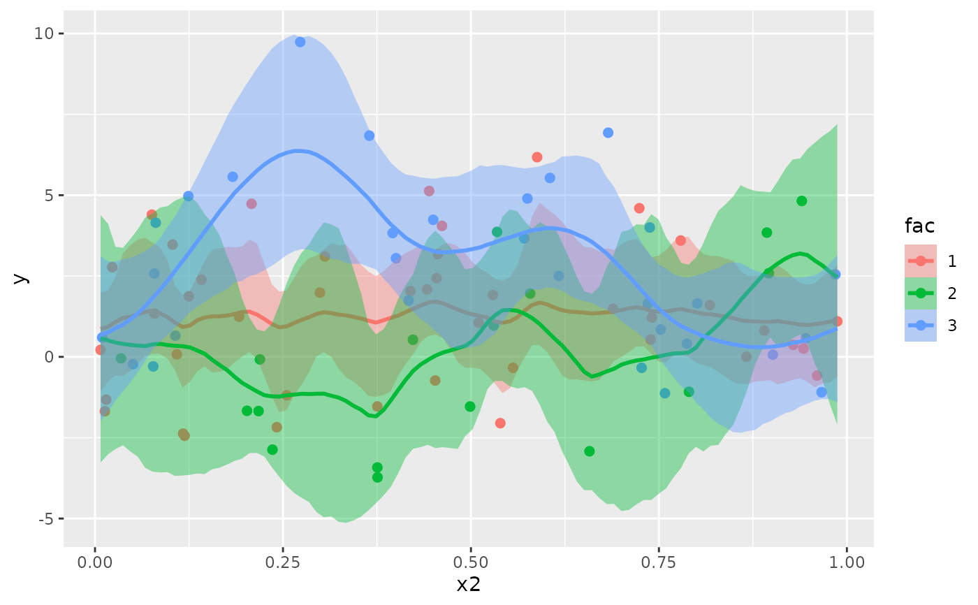
fit4 <- brm(y ~ gp(x2, by = fac), dat2, chains = 2)
#> Compiling Stan program...
#> Start sampling
#>
#> SAMPLING FOR MODEL 'anon_model' NOW (CHAIN 1).
#> Chain 1:
#> Chain 1: Gradient evaluation took 0.000166 seconds
#> Chain 1: 1000 transitions using 10 leapfrog steps per transition would take 1.66 seconds.
#> Chain 1: Adjust your expectations accordingly!
#> Chain 1:
#> Chain 1:
#> Chain 1: Iteration: 1 / 2000 [ 0%] (Warmup)
#> Chain 1: Iteration: 200 / 2000 [ 10%] (Warmup)
#> Chain 1: Iteration: 400 / 2000 [ 20%] (Warmup)
#> Chain 1: Iteration: 600 / 2000 [ 30%] (Warmup)
#> Chain 1: Iteration: 800 / 2000 [ 40%] (Warmup)
#> Chain 1: Iteration: 1000 / 2000 [ 50%] (Warmup)
#> Chain 1: Iteration: 1001 / 2000 [ 50%] (Sampling)
#> Chain 1: Iteration: 1200 / 2000 [ 60%] (Sampling)
#> Chain 1: Iteration: 1400 / 2000 [ 70%] (Sampling)
#> Chain 1: Iteration: 1600 / 2000 [ 80%] (Sampling)
#> Chain 1: Iteration: 1800 / 2000 [ 90%] (Sampling)
#> Chain 1: Iteration: 2000 / 2000 [100%] (Sampling)
#> Chain 1:
#> Chain 1: Elapsed Time: 4.033 seconds (Warm-up)
#> Chain 1: 3.822 seconds (Sampling)
#> Chain 1: 7.855 seconds (Total)
#> Chain 1:
#>
#> SAMPLING FOR MODEL 'anon_model' NOW (CHAIN 2).
#> Chain 2:
#> Chain 2: Gradient evaluation took 0.000135 seconds
#> Chain 2: 1000 transitions using 10 leapfrog steps per transition would take 1.35 seconds.
#> Chain 2: Adjust your expectations accordingly!
#> Chain 2:
#> Chain 2:
#> Chain 2: Iteration: 1 / 2000 [ 0%] (Warmup)
#> Chain 2: Iteration: 200 / 2000 [ 10%] (Warmup)
#> Chain 2: Iteration: 400 / 2000 [ 20%] (Warmup)
#> Chain 2: Iteration: 600 / 2000 [ 30%] (Warmup)
#> Chain 2: Iteration: 800 / 2000 [ 40%] (Warmup)
#> Chain 2: Iteration: 1000 / 2000 [ 50%] (Warmup)
#> Chain 2: Iteration: 1001 / 2000 [ 50%] (Sampling)
#> Chain 2: Iteration: 1200 / 2000 [ 60%] (Sampling)
#> Chain 2: Iteration: 1400 / 2000 [ 70%] (Sampling)
#> Chain 2: Iteration: 1600 / 2000 [ 80%] (Sampling)
#> Chain 2: Iteration: 1800 / 2000 [ 90%] (Sampling)
#> Chain 2: Iteration: 2000 / 2000 [100%] (Sampling)
#> Chain 2:
#> Chain 2: Elapsed Time: 4.124 seconds (Warm-up)
#> Chain 2: 3.878 seconds (Sampling)
#> Chain 2: 8.002 seconds (Total)
#> Chain 2:
#> Warning: There were 1 divergent transitions after warmup. See
#> https://mc-stan.org/misc/warnings.html#divergent-transitions-after-warmup
#> to find out why this is a problem and how to eliminate them.
#> Warning: Examine the pairs() plot to diagnose sampling problems
summary(fit4)
#> Warning: There were 1 divergent transitions after warmup. Increasing adapt_delta above 0.8 may help. See http://mc-stan.org/misc/warnings.html#divergent-transitions-after-warmup
#> Family: gaussian
#> Links: mu = identity
#> Formula: y ~ gp(x2, by = fac)
#> Data: dat2 (Number of observations: 90)
#> Draws: 2 chains, each with iter = 2000; warmup = 1000; thin = 1;
#> total post-warmup draws = 2000
#>
#> Gaussian Process Hyperparameters:
#> Estimate Est.Error l-95% CI u-95% CI Rhat Bulk_ESS Tail_ESS
#> sdgp(gpx2fac1) 0.84 0.54 0.04 1.99 1.00 464 969
#> sdgp(gpx2fac2) 2.44 0.99 0.81 4.79 1.00 816 1012
#> sdgp(gpx2fac3) 2.81 1.06 1.33 5.29 1.00 963 1300
#> lscale(gpx2fac1) 0.20 3.12 0.01 0.44 1.01 524 1064
#> lscale(gpx2fac2) 0.10 0.12 0.02 0.38 1.00 432 525
#> lscale(gpx2fac3) 0.13 0.07 0.05 0.31 1.00 582 447
#>
#> Regression Coefficients:
#> Estimate Est.Error l-95% CI u-95% CI Rhat Bulk_ESS Tail_ESS
#> Intercept 1.25 0.41 0.46 2.06 1.00 1433 1209
#>
#> Further Distributional Parameters:
#> Estimate Est.Error l-95% CI u-95% CI Rhat Bulk_ESS Tail_ESS
#> sigma 2.00 0.20 1.64 2.43 1.00 618 1081
#>
#> Draws were sampled using sampling(NUTS). For each parameter, Bulk_ESS
#> and Tail_ESS are effective sample size measures, and Rhat is the potential
#> scale reduction factor on split chains (at convergence, Rhat = 1).
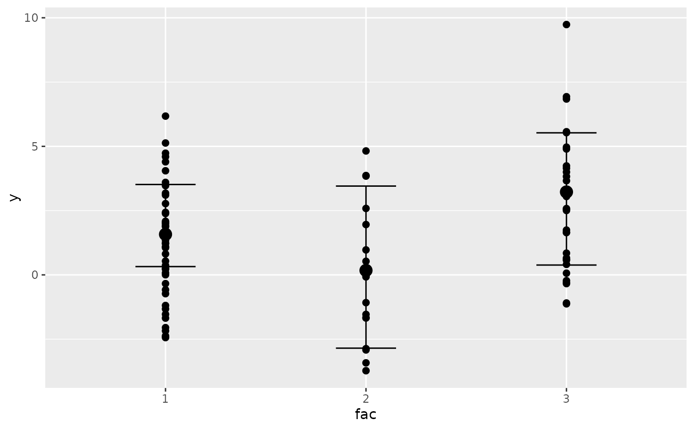
plot(conditional_effects(fit4), points = TRUE)
# compare model fit
loo(fit1, fit2, fit3)
#> Warning: Found 1 observations with a pareto_k > 0.7 in model 'fit1'. We recommend to set 'moment_match = TRUE' in order to perform moment matching for problematic observations.
#> Warning: Found 3 observations with a pareto_k > 0.7 in model 'fit2'. We recommend to set 'moment_match = TRUE' in order to perform moment matching for problematic observations.
#> Warning: Found 15 observations with a pareto_k > 0.7 in model 'fit3'. We recommend to set 'moment_match = TRUE' in order to perform moment matching for problematic observations.
#> Output of model 'fit1':
#>
#> Computed from 2000 by 30 log-likelihood matrix.
#>
#> Estimate SE
#> elpd_loo -78.0 4.7
#> p_loo 9.6 2.8
#> looic 156.0 9.3
#> ------
#> MCSE of elpd_loo is NA.
#> MCSE and ESS estimates assume MCMC draws (r_eff in [0.2, 1.1]).
#>
#> Pareto k diagnostic values:
#> Count Pct. Min. ESS
#> (-Inf, 0.7] (good) 29 96.7% 76
#> (0.7, 1] (bad) 1 3.3% <NA>
#> (1, Inf) (very bad) 0 0.0% <NA>
#> See help('pareto-k-diagnostic') for details.
#>
#> Output of model 'fit2':
#>
#> Computed from 2000 by 30 log-likelihood matrix.
#>
#> Estimate SE
#> elpd_loo -72.1 3.9
#> p_loo 10.4 2.4
#> looic 144.1 7.8
#> ------
#> MCSE of elpd_loo is NA.
#> MCSE and ESS estimates assume MCMC draws (r_eff in [0.4, 1.0]).
#>
#> Pareto k diagnostic values:
#> Count Pct. Min. ESS
#> (-Inf, 0.7] (good) 27 90.0% 290
#> (0.7, 1] (bad) 3 10.0% <NA>
#> (1, Inf) (very bad) 0 0.0% <NA>
#> See help('pareto-k-diagnostic') for details.
#>
#> Output of model 'fit3':
#>
#> Computed from 2000 by 30 log-likelihood matrix.
#>
#> Estimate SE
#> elpd_loo -70.8 4.1
#> p_loo 20.2 3.5
#> looic 141.5 8.1
#> ------
#> MCSE of elpd_loo is NA.
#> MCSE and ESS estimates assume MCMC draws (r_eff in [0.0, 0.1]).
#>
#> Pareto k diagnostic values:
#> Count Pct. Min. ESS
#> (-Inf, 0.7] (good) 15 50.0% 23
#> (0.7, 1] (bad) 13 43.3% <NA>
#> (1, Inf) (very bad) 2 6.7% <NA>
#> See help('pareto-k-diagnostic') for details.
#>
#> Model comparisons:
#> model elpd_diff se_diff p_worse diag_diff diag_elpd
#> fit3 0.0 0.0 NA 15 k_psis > 0.7
#> fit2 -1.3 2.2 0.72 N < 100 3 k_psis > 0.7
#> fit1 -7.2 2.9 0.99 N < 100 1 k_psis > 0.7
#>
#> Diagnostic flags present.
#> See ?`loo-glossary` (sections `diag_diff` and `diag_elpd`)
#> or https://mc-stan.org/loo/reference/loo-glossary.html.
# simulate data with a factor covariate
dat2 <- mgcv::gamSim(4, n = 90, scale = 2)
#> Factor `by' variable example
# fit separate gaussian processes for different levels of 'fac'
fit4 <- brm(y ~ gp(x2, by = fac), dat2, chains = 2)
#> Compiling Stan program...
#> Start sampling
#>
#> SAMPLING FOR MODEL 'anon_model' NOW (CHAIN 1).
#> Chain 1:
#> Chain 1: Gradient evaluation took 0.000166 seconds
#> Chain 1: 1000 transitions using 10 leapfrog steps per transition would take 1.66 seconds.
#> Chain 1: Adjust your expectations accordingly!
#> Chain 1:
#> Chain 1:
#> Chain 1: Iteration: 1 / 2000 [ 0%] (Warmup)
#> Chain 1: Iteration: 200 / 2000 [ 10%] (Warmup)
#> Chain 1: Iteration: 400 / 2000 [ 20%] (Warmup)
#> Chain 1: Iteration: 600 / 2000 [ 30%] (Warmup)
#> Chain 1: Iteration: 800 / 2000 [ 40%] (Warmup)
#> Chain 1: Iteration: 1000 / 2000 [ 50%] (Warmup)
#> Chain 1: Iteration: 1001 / 2000 [ 50%] (Sampling)
#> Chain 1: Iteration: 1200 / 2000 [ 60%] (Sampling)
#> Chain 1: Iteration: 1400 / 2000 [ 70%] (Sampling)
#> Chain 1: Iteration: 1600 / 2000 [ 80%] (Sampling)
#> Chain 1: Iteration: 1800 / 2000 [ 90%] (Sampling)
#> Chain 1: Iteration: 2000 / 2000 [100%] (Sampling)
#> Chain 1:
#> Chain 1: Elapsed Time: 4.033 seconds (Warm-up)
#> Chain 1: 3.822 seconds (Sampling)
#> Chain 1: 7.855 seconds (Total)
#> Chain 1:
#>
#> SAMPLING FOR MODEL 'anon_model' NOW (CHAIN 2).
#> Chain 2:
#> Chain 2: Gradient evaluation took 0.000135 seconds
#> Chain 2: 1000 transitions using 10 leapfrog steps per transition would take 1.35 seconds.
#> Chain 2: Adjust your expectations accordingly!
#> Chain 2:
#> Chain 2:
#> Chain 2: Iteration: 1 / 2000 [ 0%] (Warmup)
#> Chain 2: Iteration: 200 / 2000 [ 10%] (Warmup)
#> Chain 2: Iteration: 400 / 2000 [ 20%] (Warmup)
#> Chain 2: Iteration: 600 / 2000 [ 30%] (Warmup)
#> Chain 2: Iteration: 800 / 2000 [ 40%] (Warmup)
#> Chain 2: Iteration: 1000 / 2000 [ 50%] (Warmup)
#> Chain 2: Iteration: 1001 / 2000 [ 50%] (Sampling)
#> Chain 2: Iteration: 1200 / 2000 [ 60%] (Sampling)
#> Chain 2: Iteration: 1400 / 2000 [ 70%] (Sampling)
#> Chain 2: Iteration: 1600 / 2000 [ 80%] (Sampling)
#> Chain 2: Iteration: 1800 / 2000 [ 90%] (Sampling)
#> Chain 2: Iteration: 2000 / 2000 [100%] (Sampling)
#> Chain 2:
#> Chain 2: Elapsed Time: 4.124 seconds (Warm-up)
#> Chain 2: 3.878 seconds (Sampling)
#> Chain 2: 8.002 seconds (Total)
#> Chain 2:
#> Warning: There were 1 divergent transitions after warmup. See
#> https://mc-stan.org/misc/warnings.html#divergent-transitions-after-warmup
#> to find out why this is a problem and how to eliminate them.
#> Warning: Examine the pairs() plot to diagnose sampling problems
summary(fit4)
#> Warning: There were 1 divergent transitions after warmup. Increasing adapt_delta above 0.8 may help. See http://mc-stan.org/misc/warnings.html#divergent-transitions-after-warmup
#> Family: gaussian
#> Links: mu = identity
#> Formula: y ~ gp(x2, by = fac)
#> Data: dat2 (Number of observations: 90)
#> Draws: 2 chains, each with iter = 2000; warmup = 1000; thin = 1;
#> total post-warmup draws = 2000
#>
#> Gaussian Process Hyperparameters:
#> Estimate Est.Error l-95% CI u-95% CI Rhat Bulk_ESS Tail_ESS
#> sdgp(gpx2fac1) 0.84 0.54 0.04 1.99 1.00 464 969
#> sdgp(gpx2fac2) 2.44 0.99 0.81 4.79 1.00 816 1012
#> sdgp(gpx2fac3) 2.81 1.06 1.33 5.29 1.00 963 1300
#> lscale(gpx2fac1) 0.20 3.12 0.01 0.44 1.01 524 1064
#> lscale(gpx2fac2) 0.10 0.12 0.02 0.38 1.00 432 525
#> lscale(gpx2fac3) 0.13 0.07 0.05 0.31 1.00 582 447
#>
#> Regression Coefficients:
#> Estimate Est.Error l-95% CI u-95% CI Rhat Bulk_ESS Tail_ESS
#> Intercept 1.25 0.41 0.46 2.06 1.00 1433 1209
#>
#> Further Distributional Parameters:
#> Estimate Est.Error l-95% CI u-95% CI Rhat Bulk_ESS Tail_ESS
#> sigma 2.00 0.20 1.64 2.43 1.00 618 1081
#>
#> Draws were sampled using sampling(NUTS). For each parameter, Bulk_ESS
#> and Tail_ESS are effective sample size measures, and Rhat is the potential
#> scale reduction factor on split chains (at convergence, Rhat = 1).
plot(conditional_effects(fit4), points = TRUE)
 # }
# }