(Deprecated) Spatial simultaneous autoregressive (SAR) structures

Thse functions are deprecated. Please see sar for the new syntax. These functions are constructors for the cor_sar class implementing spatial simultaneous autoregressive structures. The lagsar structure implements SAR of the response values: $$y = \rho W y + \eta + e$$ The errorsar structure implements SAR of the residuals: $$y = \eta + u, u = \rho W u + e$$ In the above equations, \(\eta\) is the predictor term and \(e\) are independent normally or t-distributed residuals.

Usage

cor_sar(W, type = c("lag", "error"))

cor_lagsar(W)

cor_errorsar(W)

Arguments

W

An object specifying the spatial weighting matrix. Can be either the spatial weight matrix itself or an object of class listw or nb, from which the spatial weighting matrix can be computed.

type

Type of the SAR structure. Either "lag" (for SAR of the response values) or "error" (for SAR of the residuals).

Value

An object of class cor_sar to be used in calls to brm.

Details

Currently, only families gaussian and student support SAR structures.

Examples

# \dontrun{
data(oldcol, package = "spdep")
fit1 <- brm(CRIME ~ INC + HOVAL, data = COL.OLD,
            autocor = cor_lagsar(COL.nb),
            chains = 2, cores = 2)
#> Warning: Argument 'autocor' should be specified within the 'formula' argument. See ?brmsformula for help.
#> Warning: Using 'cor_brms' objects for 'autocor' is deprecated. Please see ?cor_brms for details.
#> Compiling Stan program...
#> Start sampling
summary(fit1)
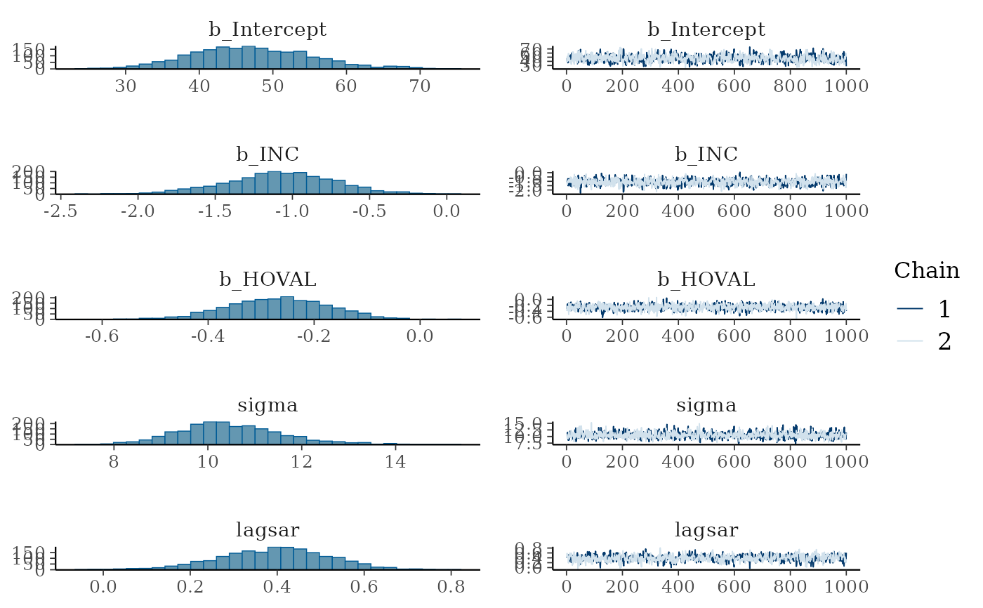
plot(fit1)


fit2 <- brm(CRIME ~ INC + HOVAL, data = COL.OLD,
            autocor = cor_errorsar(COL.nb),
            chains = 2, cores = 2)
#> Warning: Argument 'autocor' should be specified within the 'formula' argument. See ?brmsformula for help.
#> Warning: Using 'cor_brms' objects for 'autocor' is deprecated. Please see ?cor_brms for details.
#> Compiling Stan program...
#> Start sampling
summary(fit2)
#>  -0.99      0.40    -1.77    -0.21 1.00     1006     1103
#> HOVAL        -0.29      0.10    -0.49    -0.10 1.00     1272     1282
#> 
#> Further Distributional Parameters:
#>       Estimate Est.Error l-95% CI u-95% CI Rhat Bulk_ESS Tail_ESS
#> sigma    10.37      1.14     8.38    12.76 1.00     1928     1195
#> 
#> Draws were sampled using sampling(NUTS). For each parameter, Bulk_ESS
#> and Tail_ESS are effective sample size measures, and Rhat is the potential
#> scale reduction factor on split chains (at convergence, Rhat = 1).
#> n: 1600 / 2000 [ 80%]  (Sampling)
#> Chain 1: Iteration: 1600 / 2000 [ 80%]  (Sampling)
#> Chain 2: Iteration: 1800 / 2000 [ 90%]  (Sampling)
#> Chain 1: Iteration: 1800 / 2000 [ 90%]  (Sampling)
#> Chain 2: Iteration: 2000 / 2000 [100%]  (Sampling)
#> Chain 2: 
#> Chain 2:  Elapsed Time: 0.378 seconds (Warm-up)
#> Chain 2:                0.271 seconds (Sampling)
#> Chain 2:                0.649 seconds (Total)
#> Chain 2: 
#> Chain 1: Iteration: 2000 / 2000 [100%]  (Sampling)
#> Chain 1: 
#> Chain 1:  Elapsed Time: 0.423 seconds (Warm-up)
#> Chain 1:                0.258 seconds (Sampling)
#> Chain 1:                0.681 seconds (Total)
#> Chain 1: 
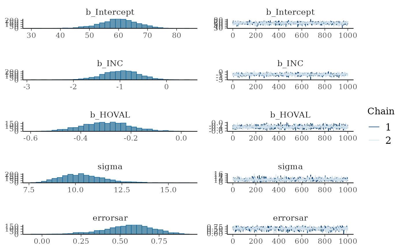
plot(fit2)

# }