
Set up an spatial simultaneous autoregressive (SAR) term in brms. The function does not evaluate its arguments – it exists purely to help set up a model with SAR terms.
Arguments
- M
An object specifying the spatial weighting matrix. Can be either the spatial weight matrix itself or an object of class
listwornb, from which the spatial weighting matrix can be computed.- type
Type of the SAR structure. Either
"lag"(for SAR of the response values) or"error"(for SAR of the residuals). More information is provided in the 'Details' section.
Value
An object of class 'sar_term', which is a list
of arguments to be interpreted by the formula
parsing functions of brms.
Details
The lagsar structure implements SAR of the response values:
$$y = \rho W y + \eta + e$$
The errorsar structure implements SAR of the residuals:
$$y = \eta + u, u = \rho W u + e$$
In the above equations, \(\eta\) is the predictor term and \(e\) are
independent normally or t-distributed residuals. Currently, only families
gaussian and student support SAR structures.
Examples
# \dontrun{
data(oldcol, package = "spdep")
fit1 <- brm(CRIME ~ INC + HOVAL + sar(COL.nb, type = "lag"),
data = COL.OLD, data2 = list(COL.nb = COL.nb),
chains = 2, cores = 2)
#> Compiling Stan program...
#> Start sampling
summary(fit1)
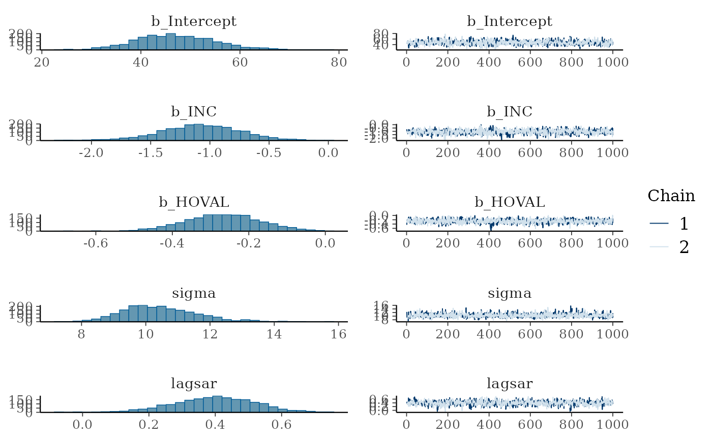
plot(fit1)
 fit2 <- brm(CRIME ~ INC + HOVAL + sar(COL.nb, type = "error"),
data = COL.OLD, data2 = list(COL.nb = COL.nb),
chains = 2, cores = 2)
#> Compiling Stan program...
#> Start sampling
summary(fit2)
#> 999 1124
#> HOVAL -0.30 0.10 -0.49 -0.11 1.00 1827 1429
#>
#> Further Distributional Parameters:
#> Estimate Est.Error l-95% CI u-95% CI Rhat Bulk_ESS Tail_ESS
#> sigma 10.36 1.14 8.39 12.85 1.00 1932 1327
#>
#> Draws were sampled using sampling(NUTS). For each parameter, Bulk_ESS
#> and Tail_ESS are effective sample size measures, and Rhat is the potential
#> scale reduction factor on split chains (at convergence, Rhat = 1).
#> ng)
#> Chain 1: Iteration: 1800 / 2000 [ 90%] (Sampling)
#> Chain 2: Iteration: 1400 / 2000 [ 70%] (Sampling)
#> Chain 1: Iteration: 2000 / 2000 [100%] (Sampling)
#> Chain 1:
#> Chain 1: Elapsed Time: 0.575 seconds (Warm-up)
#> Chain 1: 0.371 seconds (Sampling)
#> Chain 1: 0.946 seconds (Total)
#> Chain 1:
#> Chain 2: Iteration: 1600 / 2000 [ 80%] (Sampling)
#> Chain 2: Iteration: 1800 / 2000 [ 90%] (Sampling)
#> Chain 2: Iteration: 2000 / 2000 [100%] (Sampling)
#> Chain 2:
#> Chain 2: Elapsed Time: 0.623 seconds (Warm-up)
#> Chain 2: 0.48 seconds (Sampling)
#> Chain 2: 1.103 seconds (Total)
#> Chain 2:
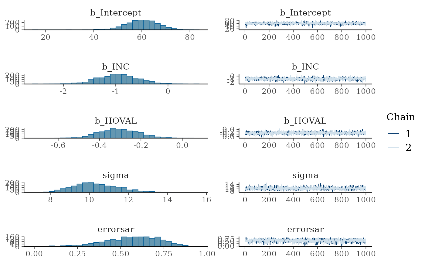
plot(fit2)
fit2 <- brm(CRIME ~ INC + HOVAL + sar(COL.nb, type = "error"),
data = COL.OLD, data2 = list(COL.nb = COL.nb),
chains = 2, cores = 2)
#> Compiling Stan program...
#> Start sampling
summary(fit2)
#> 999 1124
#> HOVAL -0.30 0.10 -0.49 -0.11 1.00 1827 1429
#>
#> Further Distributional Parameters:
#> Estimate Est.Error l-95% CI u-95% CI Rhat Bulk_ESS Tail_ESS
#> sigma 10.36 1.14 8.39 12.85 1.00 1932 1327
#>
#> Draws were sampled using sampling(NUTS). For each parameter, Bulk_ESS
#> and Tail_ESS are effective sample size measures, and Rhat is the potential
#> scale reduction factor on split chains (at convergence, Rhat = 1).
#> ng)
#> Chain 1: Iteration: 1800 / 2000 [ 90%] (Sampling)
#> Chain 2: Iteration: 1400 / 2000 [ 70%] (Sampling)
#> Chain 1: Iteration: 2000 / 2000 [100%] (Sampling)
#> Chain 1:
#> Chain 1: Elapsed Time: 0.575 seconds (Warm-up)
#> Chain 1: 0.371 seconds (Sampling)
#> Chain 1: 0.946 seconds (Total)
#> Chain 1:
#> Chain 2: Iteration: 1600 / 2000 [ 80%] (Sampling)
#> Chain 2: Iteration: 1800 / 2000 [ 90%] (Sampling)
#> Chain 2: Iteration: 2000 / 2000 [100%] (Sampling)
#> Chain 2:
#> Chain 2: Elapsed Time: 0.623 seconds (Warm-up)
#> Chain 2: 0.48 seconds (Sampling)
#> Chain 2: 1.103 seconds (Total)
#> Chain 2:
plot(fit2)
 # }
# }