
Set up a finite mixture family for use in brms.
Arguments
- ...
One or more objects providing a description of the response distributions to be combined in the mixture model. These can be family functions, calls to family functions or character strings naming the families. For details of supported families see
brmsfamily.- flist
Optional list of objects, which are treated in the same way as objects passed via the
...argument.- nmix
Optional numeric vector specifying the number of times each family is repeated. If specified, it must have the same length as the number of families passed via
...andflist.- order
Ordering constraint to identify mixture components. If
'mu'orTRUE, population-level intercepts of the mean parameters are ordered in non-ordinal models and fixed to the same value in ordinal models (see details). If'none'orFALSE, no ordering constraint is applied. IfNULL(the default),orderis set to'mu'if all families are the same and'none'otherwise. Other ordering constraints may be implemented in the future.- refcat
Optional reference category for the mixing proportions. By default (
NULL), when the mixing proportions are predicted, all but one of them have to be modeled while the remaining one serves as the reference category (its linear predictor is fixed to zero) to identify the model. Ifrefcat = NA, no reference category is used and all mixing proportions are predicted via a 'softmax' transformation. This is analogous torefcat = NAincategoricalmodels. As the resulting model is only weakly identified, informative priors on thethetaparameters are strongly recommended (see the examples inbrmsformula).
Details
Most families supported by brms can be used to form mixtures. The response variable has to be valid for all components of the mixture family. Currently, the number of mixture components has to be specified by the user. It is not yet possible to estimate the number of mixture components from the data.
Ordering intercepts in mixtures of ordinal families is not possible as each family has itself a set of vector of intercepts (i.e. ordinal thresholds). Instead, brms will fix the vector of intercepts across components in ordinal mixtures, if desired, so that users can try to identify the mixture model via selective inclusion of predictors.
For most mixture models, you may want to specify priors on the
population-level intercepts via set_prior to improve
posterior inference. In addition, it is sometimes necessary to set init = 0
in the call to brm to allow chains to initialize properly.
For more details on the specification of mixture
models, see brmsformula.
Examples
# \dontrun{
## simulate some data
set.seed(1234)
dat <- data.frame(
y = c(rnorm(200), rnorm(100, 6)),
x = rnorm(300),
z = sample(0:1, 300, TRUE)
)
## fit a simple normal mixture model
mix <- mixture(gaussian, gaussian)
#> Setting order = 'mu' for mixtures of the same family.
prior <- c(
prior(normal(0, 7), Intercept, dpar = mu1),
prior(normal(5, 7), Intercept, dpar = mu2)
)
fit1 <- brm(bf(y ~ x + z), dat, family = mix,
prior = prior, chains = 2)
#> Compiling Stan program...
#> Start sampling
#>
#> SAMPLING FOR MODEL 'anon_model' NOW (CHAIN 1).
#> Chain 1:
#> Chain 1: Gradient evaluation took 0.000204 seconds
#> Chain 1: 1000 transitions using 10 leapfrog steps per transition would take 2.04 seconds.
#> Chain 1: Adjust your expectations accordingly!
#> Chain 1:
#> Chain 1:
#> Chain 1: Iteration: 1 / 2000 [ 0%] (Warmup)
#> Chain 1: Iteration: 200 / 2000 [ 10%] (Warmup)
#> Chain 1: Iteration: 400 / 2000 [ 20%] (Warmup)
#> Chain 1: Iteration: 600 / 2000 [ 30%] (Warmup)
#> Chain 1: Iteration: 800 / 2000 [ 40%] (Warmup)
#> Chain 1: Iteration: 1000 / 2000 [ 50%] (Warmup)
#> Chain 1: Iteration: 1001 / 2000 [ 50%] (Sampling)
#> Chain 1: Iteration: 1200 / 2000 [ 60%] (Sampling)
#> Chain 1: Iteration: 1400 / 2000 [ 70%] (Sampling)
#> Chain 1: Iteration: 1600 / 2000 [ 80%] (Sampling)
#> Chain 1: Iteration: 1800 / 2000 [ 90%] (Sampling)
#> Chain 1: Iteration: 2000 / 2000 [100%] (Sampling)
#> Chain 1:
#> Chain 1: Elapsed Time: 1.371 seconds (Warm-up)
#> Chain 1: 1.033 seconds (Sampling)
#> Chain 1: 2.404 seconds (Total)
#> Chain 1:
#>
#> SAMPLING FOR MODEL 'anon_model' NOW (CHAIN 2).
#> Chain 2:
#> Chain 2: Gradient evaluation took 0.000137 seconds
#> Chain 2: 1000 transitions using 10 leapfrog steps per transition would take 1.37 seconds.
#> Chain 2: Adjust your expectations accordingly!
#> Chain 2:
#> Chain 2:
#> Chain 2: Iteration: 1 / 2000 [ 0%] (Warmup)
#> Chain 2: Iteration: 200 / 2000 [ 10%] (Warmup)
#> Chain 2: Iteration: 400 / 2000 [ 20%] (Warmup)
#> Chain 2: Iteration: 600 / 2000 [ 30%] (Warmup)
#> Chain 2: Iteration: 800 / 2000 [ 40%] (Warmup)
#> Chain 2: Iteration: 1000 / 2000 [ 50%] (Warmup)
#> Chain 2: Iteration: 1001 / 2000 [ 50%] (Sampling)
#> Chain 2: Iteration: 1200 / 2000 [ 60%] (Sampling)
#> Chain 2: Iteration: 1400 / 2000 [ 70%] (Sampling)
#> Chain 2: Iteration: 1600 / 2000 [ 80%] (Sampling)
#> Chain 2: Iteration: 1800 / 2000 [ 90%] (Sampling)
#> Chain 2: Iteration: 2000 / 2000 [100%] (Sampling)
#> Chain 2:
#> Chain 2: Elapsed Time: 29.819 seconds (Warm-up)
#> Chain 2: 43.637 seconds (Sampling)
#> Chain 2: 73.456 seconds (Total)
#> Chain 2:
#> Warning: There were 241 transitions after warmup that exceeded the maximum treedepth. Increase max_treedepth above 10. See
#> https://mc-stan.org/misc/warnings.html#maximum-treedepth-exceeded
#> Warning: Examine the pairs() plot to diagnose sampling problems
#> Warning: The largest R-hat is 2.98, indicating chains have not mixed.
#> Running the chains for more iterations may help. See
#> https://mc-stan.org/misc/warnings.html#r-hat
#> Warning: Bulk Effective Samples Size (ESS) is too low, indicating posterior means and medians may be unreliable.
#> Running the chains for more iterations may help. See
#> https://mc-stan.org/misc/warnings.html#bulk-ess
#> Warning: Tail Effective Samples Size (ESS) is too low, indicating posterior variances and tail quantiles may be unreliable.
#> Running the chains for more iterations may help. See
#> https://mc-stan.org/misc/warnings.html#tail-ess
summary(fit1)
#> Warning: Inference for the model posterior has not converged (some Rhats are > 1.05). Be careful when analysing the results! We recommend running more iterations or setting stronger priors.
#> Family: mixture(gaussian, gaussian)
#> Links: mu1 = identity; mu2 = identity
#> Formula: y ~ x + z
#> Data: dat (Number of observations: 300)
#> Draws: 2 chains, each with iter = 2000; warmup = 1000; thin = 1;
#> total post-warmup draws = 2000
#>
#> Regression Coefficients:
#> Estimate Est.Error l-95% CI
#> mu1_Intercept 1.27 1.23 -0.14
#> mu2_Intercept 35465969799385544.00 41709491594432400.00 6.00
#> mu1_x -0.03 0.17 -0.43
#> mu1_z -0.53 0.45 -1.47
#> mu2_x -1029595764310982.50 2668856112243263.50 -7786776878225666.00
#> mu2_z -64981471364136320.00 76404249972577952.00 -210153805226743360.00
#> u-95% CI Rhat Bulk_ESS Tail_ESS
#> mu1_Intercept 2.94 1.83 3 101
#> mu2_Intercept 114609037117292896.00 2.45 3 27
#> mu1_x 0.21 1.18 8 84
#> mu1_z 0.08 1.66 3 71
#> mu2_x 3923343878003977.00 1.85 25 48
#> mu2_z 0.20 2.98 3 27
#>
#> Further Distributional Parameters:
#> Estimate Est.Error l-95% CI u-95% CI Rhat Bulk_ESS Tail_ESS
#> sigma1 2.06 1.03 0.96 3.29 1.83 3 73
#> sigma2 1.82 2.15 0.19 7.93 1.60 23 61
#> theta1 0.83 0.17 0.62 1.00 1.83 3 62
#> theta2 0.17 0.17 0.00 0.38 1.83 3 62
#>
#> Draws were sampled using sampling(NUTS). For each parameter, Bulk_ESS
#> and Tail_ESS are effective sample size measures, and Rhat is the potential
#> scale reduction factor on split chains (at convergence, Rhat = 1).
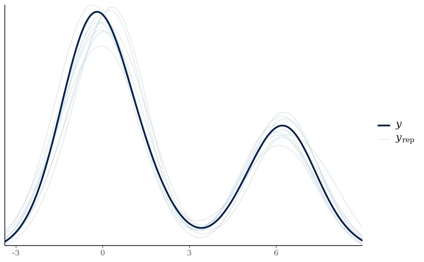
pp_check(fit1)
#> Using 10 posterior draws for ppc type 'dens_overlay' by default.
 ## use different predictors for the components
fit2 <- brm(bf(y ~ 1, mu1 ~ x, mu2 ~ z), dat, family = mix,
prior = prior, chains = 2)
#> Compiling Stan program...
#> Start sampling
#>
#> SAMPLING FOR MODEL 'anon_model' NOW (CHAIN 1).
#> Chain 1:
#> Chain 1: Gradient evaluation took 0.000151 seconds
#> Chain 1: 1000 transitions using 10 leapfrog steps per transition would take 1.51 seconds.
#> Chain 1: Adjust your expectations accordingly!
#> Chain 1:
#> Chain 1:
#> Chain 1: Iteration: 1 / 2000 [ 0%] (Warmup)
#> Chain 1: Iteration: 200 / 2000 [ 10%] (Warmup)
#> Chain 1: Iteration: 400 / 2000 [ 20%] (Warmup)
#> Chain 1: Iteration: 600 / 2000 [ 30%] (Warmup)
#> Chain 1: Iteration: 800 / 2000 [ 40%] (Warmup)
#> Chain 1: Iteration: 1000 / 2000 [ 50%] (Warmup)
#> Chain 1: Iteration: 1001 / 2000 [ 50%] (Sampling)
#> Chain 1: Iteration: 1200 / 2000 [ 60%] (Sampling)
#> Chain 1: Iteration: 1400 / 2000 [ 70%] (Sampling)
#> Chain 1: Iteration: 1600 / 2000 [ 80%] (Sampling)
#> Chain 1: Iteration: 1800 / 2000 [ 90%] (Sampling)
#> Chain 1: Iteration: 2000 / 2000 [100%] (Sampling)
#> Chain 1:
#> Chain 1: Elapsed Time: 1.284 seconds (Warm-up)
#> Chain 1: 1.018 seconds (Sampling)
#> Chain 1: 2.302 seconds (Total)
#> Chain 1:
#>
#> SAMPLING FOR MODEL 'anon_model' NOW (CHAIN 2).
#> Chain 2:
#> Chain 2: Gradient evaluation took 0.000134 seconds
#> Chain 2: 1000 transitions using 10 leapfrog steps per transition would take 1.34 seconds.
#> Chain 2: Adjust your expectations accordingly!
#> Chain 2:
#> Chain 2:
#> Chain 2: Iteration: 1 / 2000 [ 0%] (Warmup)
#> Chain 2: Iteration: 200 / 2000 [ 10%] (Warmup)
#> Chain 2: Iteration: 400 / 2000 [ 20%] (Warmup)
#> Chain 2: Iteration: 600 / 2000 [ 30%] (Warmup)
#> Chain 2: Iteration: 800 / 2000 [ 40%] (Warmup)
#> Chain 2: Iteration: 1000 / 2000 [ 50%] (Warmup)
#> Chain 2: Iteration: 1001 / 2000 [ 50%] (Sampling)
#> Chain 2: Iteration: 1200 / 2000 [ 60%] (Sampling)
#> Chain 2: Iteration: 1400 / 2000 [ 70%] (Sampling)
#> Chain 2: Iteration: 1600 / 2000 [ 80%] (Sampling)
#> Chain 2: Iteration: 1800 / 2000 [ 90%] (Sampling)
#> Chain 2: Iteration: 2000 / 2000 [100%] (Sampling)
#> Chain 2:
#> Chain 2: Elapsed Time: 1.439 seconds (Warm-up)
#> Chain 2: 1.036 seconds (Sampling)
#> Chain 2: 2.475 seconds (Total)
#> Chain 2:
#> Warning: There were 1 divergent transitions after warmup. See
#> https://mc-stan.org/misc/warnings.html#divergent-transitions-after-warmup
#> to find out why this is a problem and how to eliminate them.
#> Warning: Examine the pairs() plot to diagnose sampling problems
#> Warning: The largest R-hat is 1.83, indicating chains have not mixed.
#> Running the chains for more iterations may help. See
#> https://mc-stan.org/misc/warnings.html#r-hat
#> Warning: Bulk Effective Samples Size (ESS) is too low, indicating posterior means and medians may be unreliable.
#> Running the chains for more iterations may help. See
#> https://mc-stan.org/misc/warnings.html#bulk-ess
#> Warning: Tail Effective Samples Size (ESS) is too low, indicating posterior variances and tail quantiles may be unreliable.
#> Running the chains for more iterations may help. See
#> https://mc-stan.org/misc/warnings.html#tail-ess
summary(fit2)
#> Warning: Inference for the model posterior has not converged (some Rhats are > 1.05). Be careful when analysing the results! We recommend running more iterations or setting stronger priors.
#> Warning: There were 1 divergent transitions after warmup. Increasing adapt_delta above 0.8 may help. See http://mc-stan.org/misc/warnings.html#divergent-transitions-after-warmup
#> Family: mixture(gaussian, gaussian)
#> Links: mu1 = identity; mu2 = identity
#> Formula: y ~ 1
#> mu1 ~ x
#> mu2 ~ z
#> Data: dat (Number of observations: 300)
#> Draws: 2 chains, each with iter = 2000; warmup = 1000; thin = 1;
#> total post-warmup draws = 2000
#>
#> Regression Coefficients:
#> Estimate Est.Error l-95% CI u-95% CI Rhat Bulk_ESS Tail_ESS
#> mu1_Intercept -0.04 0.09 -0.21 0.13 1.02 2001 1158
#> mu2_Intercept 3.19 3.04 -0.06 6.44 1.83 3 69
#> mu1_x -0.11 0.33 -0.95 0.34 1.36 10 78
#> mu2_z -0.17 0.19 -0.55 0.22 1.12 11 276
#>
#> Further Distributional Parameters:
#> Estimate Est.Error l-95% CI u-95% CI Rhat Bulk_ESS Tail_ESS
#> sigma1 3.03 2.01 0.96 5.60 1.83 3 54
#> sigma2 0.85 0.11 0.65 1.05 1.54 4 76
#> theta1 0.60 0.07 0.47 0.71 1.80 3 69
#> theta2 0.40 0.07 0.29 0.53 1.80 3 69
#>
#> Draws were sampled using sampling(NUTS). For each parameter, Bulk_ESS
#> and Tail_ESS are effective sample size measures, and Rhat is the potential
#> scale reduction factor on split chains (at convergence, Rhat = 1).
## fix the mixing proportions
fit3 <- brm(bf(y ~ x + z, theta1 = 1, theta2 = 2),
dat, family = mix, prior = prior,
init = 0, chains = 2)
#> Compiling Stan program...
#> Start sampling
#>
#> SAMPLING FOR MODEL 'anon_model' NOW (CHAIN 1).
#> Chain 1:
#> Chain 1: Gradient evaluation took 0.000127 seconds
#> Chain 1: 1000 transitions using 10 leapfrog steps per transition would take 1.27 seconds.
#> Chain 1: Adjust your expectations accordingly!
#> Chain 1:
#> Chain 1:
#> Chain 1: Iteration: 1 / 2000 [ 0%] (Warmup)
#> Chain 1: Iteration: 200 / 2000 [ 10%] (Warmup)
#> Chain 1: Iteration: 400 / 2000 [ 20%] (Warmup)
#> Chain 1: Iteration: 600 / 2000 [ 30%] (Warmup)
#> Chain 1: Iteration: 800 / 2000 [ 40%] (Warmup)
#> Chain 1: Iteration: 1000 / 2000 [ 50%] (Warmup)
#> Chain 1: Iteration: 1001 / 2000 [ 50%] (Sampling)
#> Chain 1: Iteration: 1200 / 2000 [ 60%] (Sampling)
#> Chain 1: Iteration: 1400 / 2000 [ 70%] (Sampling)
#> Chain 1: Iteration: 1600 / 2000 [ 80%] (Sampling)
#> Chain 1: Iteration: 1800 / 2000 [ 90%] (Sampling)
#> Chain 1: Iteration: 2000 / 2000 [100%] (Sampling)
#> Chain 1:
#> Chain 1: Elapsed Time: 1.048 seconds (Warm-up)
#> Chain 1: 0.943 seconds (Sampling)
#> Chain 1: 1.991 seconds (Total)
#> Chain 1:
#>
#> SAMPLING FOR MODEL 'anon_model' NOW (CHAIN 2).
#> Chain 2:
#> Chain 2: Gradient evaluation took 0.000123 seconds
#> Chain 2: 1000 transitions using 10 leapfrog steps per transition would take 1.23 seconds.
#> Chain 2: Adjust your expectations accordingly!
#> Chain 2:
#> Chain 2:
#> Chain 2: Iteration: 1 / 2000 [ 0%] (Warmup)
#> Chain 2: Iteration: 200 / 2000 [ 10%] (Warmup)
#> Chain 2: Iteration: 400 / 2000 [ 20%] (Warmup)
#> Chain 2: Iteration: 600 / 2000 [ 30%] (Warmup)
#> Chain 2: Iteration: 800 / 2000 [ 40%] (Warmup)
#> Chain 2: Iteration: 1000 / 2000 [ 50%] (Warmup)
#> Chain 2: Iteration: 1001 / 2000 [ 50%] (Sampling)
#> Chain 2: Iteration: 1200 / 2000 [ 60%] (Sampling)
#> Chain 2: Iteration: 1400 / 2000 [ 70%] (Sampling)
#> Chain 2: Iteration: 1600 / 2000 [ 80%] (Sampling)
#> Chain 2: Iteration: 1800 / 2000 [ 90%] (Sampling)
#> Chain 2: Iteration: 2000 / 2000 [100%] (Sampling)
#> Chain 2:
#> Chain 2: Elapsed Time: 1.032 seconds (Warm-up)
#> Chain 2: 0.877 seconds (Sampling)
#> Chain 2: 1.909 seconds (Total)
#> Chain 2:
summary(fit3)
#> Family: mixture(gaussian, gaussian)
#> Links: mu1 = identity; mu2 = identity
#> Formula: y ~ x + z
#> theta1 = 0.33
#> theta2 = 0.67
#> Data: dat (Number of observations: 300)
#> Draws: 2 chains, each with iter = 2000; warmup = 1000; thin = 1;
#> total post-warmup draws = 2000
#>
#> Regression Coefficients:
#> Estimate Est.Error l-95% CI u-95% CI Rhat Bulk_ESS Tail_ESS
#> mu1_Intercept -0.19 0.11 -0.41 0.01 1.00 3052 1809
#> mu2_Intercept 4.49 0.45 3.61 5.34 1.00 2983 1642
#> mu1_x -0.01 0.08 -0.15 0.15 1.00 3496 1594
#> mu1_z -0.23 0.15 -0.51 0.08 1.00 3365 1739
#> mu2_x -0.22 0.28 -0.77 0.32 1.00 2940 1637
#> mu2_z -1.28 0.57 -2.41 -0.10 1.00 2432 1418
#>
#> Further Distributional Parameters:
#> Estimate Est.Error l-95% CI u-95% CI Rhat Bulk_ESS Tail_ESS
#> sigma1 0.68 0.06 0.56 0.81 1.00 2862 1639
#> sigma2 2.98 0.19 2.64 3.35 1.00 2422 1515
#>
#> Draws were sampled using sampling(NUTS). For each parameter, Bulk_ESS
#> and Tail_ESS are effective sample size measures, and Rhat is the potential
#> scale reduction factor on split chains (at convergence, Rhat = 1).
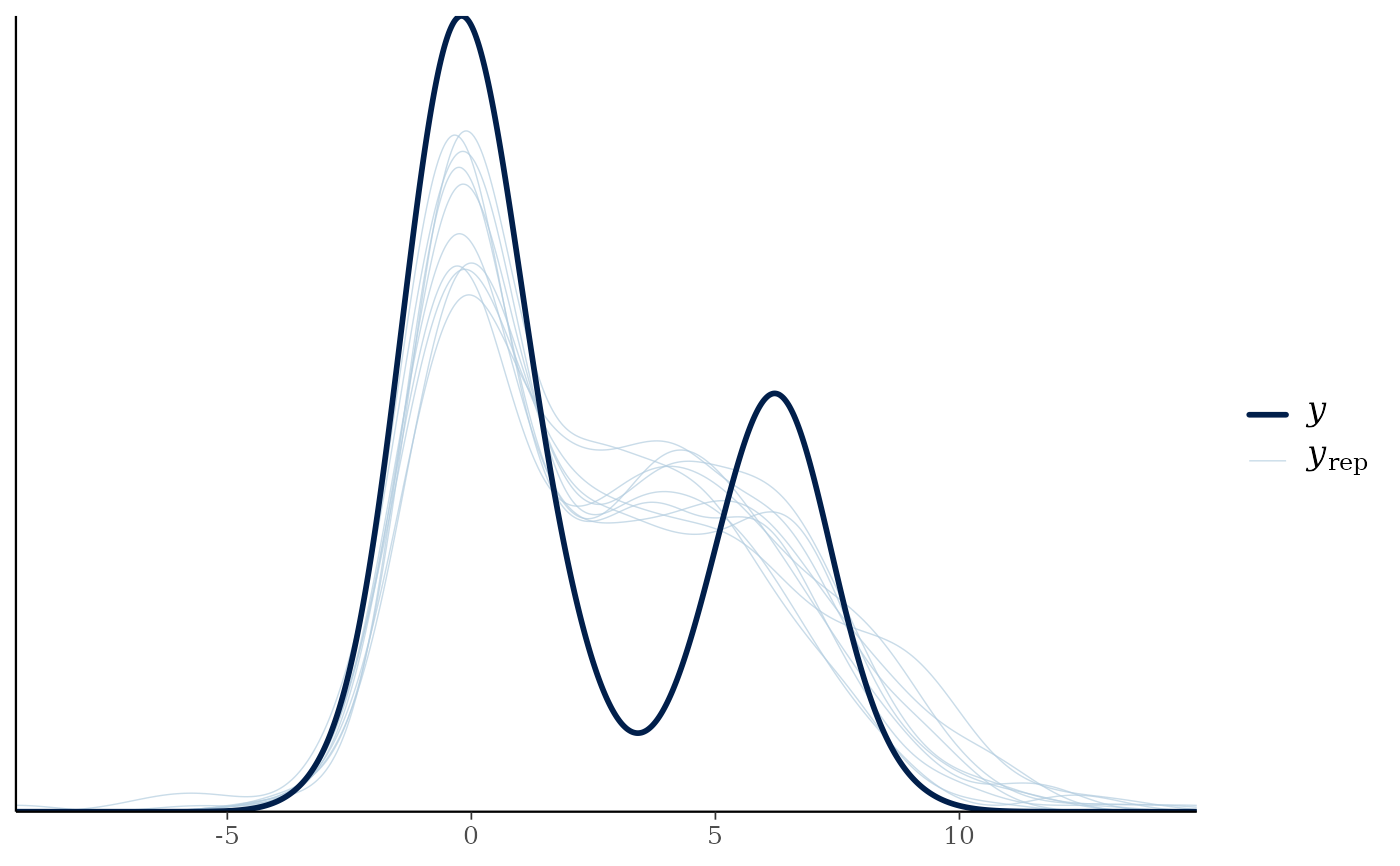
pp_check(fit3)
#> Using 10 posterior draws for ppc type 'dens_overlay' by default.
## use different predictors for the components
fit2 <- brm(bf(y ~ 1, mu1 ~ x, mu2 ~ z), dat, family = mix,
prior = prior, chains = 2)
#> Compiling Stan program...
#> Start sampling
#>
#> SAMPLING FOR MODEL 'anon_model' NOW (CHAIN 1).
#> Chain 1:
#> Chain 1: Gradient evaluation took 0.000151 seconds
#> Chain 1: 1000 transitions using 10 leapfrog steps per transition would take 1.51 seconds.
#> Chain 1: Adjust your expectations accordingly!
#> Chain 1:
#> Chain 1:
#> Chain 1: Iteration: 1 / 2000 [ 0%] (Warmup)
#> Chain 1: Iteration: 200 / 2000 [ 10%] (Warmup)
#> Chain 1: Iteration: 400 / 2000 [ 20%] (Warmup)
#> Chain 1: Iteration: 600 / 2000 [ 30%] (Warmup)
#> Chain 1: Iteration: 800 / 2000 [ 40%] (Warmup)
#> Chain 1: Iteration: 1000 / 2000 [ 50%] (Warmup)
#> Chain 1: Iteration: 1001 / 2000 [ 50%] (Sampling)
#> Chain 1: Iteration: 1200 / 2000 [ 60%] (Sampling)
#> Chain 1: Iteration: 1400 / 2000 [ 70%] (Sampling)
#> Chain 1: Iteration: 1600 / 2000 [ 80%] (Sampling)
#> Chain 1: Iteration: 1800 / 2000 [ 90%] (Sampling)
#> Chain 1: Iteration: 2000 / 2000 [100%] (Sampling)
#> Chain 1:
#> Chain 1: Elapsed Time: 1.284 seconds (Warm-up)
#> Chain 1: 1.018 seconds (Sampling)
#> Chain 1: 2.302 seconds (Total)
#> Chain 1:
#>
#> SAMPLING FOR MODEL 'anon_model' NOW (CHAIN 2).
#> Chain 2:
#> Chain 2: Gradient evaluation took 0.000134 seconds
#> Chain 2: 1000 transitions using 10 leapfrog steps per transition would take 1.34 seconds.
#> Chain 2: Adjust your expectations accordingly!
#> Chain 2:
#> Chain 2:
#> Chain 2: Iteration: 1 / 2000 [ 0%] (Warmup)
#> Chain 2: Iteration: 200 / 2000 [ 10%] (Warmup)
#> Chain 2: Iteration: 400 / 2000 [ 20%] (Warmup)
#> Chain 2: Iteration: 600 / 2000 [ 30%] (Warmup)
#> Chain 2: Iteration: 800 / 2000 [ 40%] (Warmup)
#> Chain 2: Iteration: 1000 / 2000 [ 50%] (Warmup)
#> Chain 2: Iteration: 1001 / 2000 [ 50%] (Sampling)
#> Chain 2: Iteration: 1200 / 2000 [ 60%] (Sampling)
#> Chain 2: Iteration: 1400 / 2000 [ 70%] (Sampling)
#> Chain 2: Iteration: 1600 / 2000 [ 80%] (Sampling)
#> Chain 2: Iteration: 1800 / 2000 [ 90%] (Sampling)
#> Chain 2: Iteration: 2000 / 2000 [100%] (Sampling)
#> Chain 2:
#> Chain 2: Elapsed Time: 1.439 seconds (Warm-up)
#> Chain 2: 1.036 seconds (Sampling)
#> Chain 2: 2.475 seconds (Total)
#> Chain 2:
#> Warning: There were 1 divergent transitions after warmup. See
#> https://mc-stan.org/misc/warnings.html#divergent-transitions-after-warmup
#> to find out why this is a problem and how to eliminate them.
#> Warning: Examine the pairs() plot to diagnose sampling problems
#> Warning: The largest R-hat is 1.83, indicating chains have not mixed.
#> Running the chains for more iterations may help. See
#> https://mc-stan.org/misc/warnings.html#r-hat
#> Warning: Bulk Effective Samples Size (ESS) is too low, indicating posterior means and medians may be unreliable.
#> Running the chains for more iterations may help. See
#> https://mc-stan.org/misc/warnings.html#bulk-ess
#> Warning: Tail Effective Samples Size (ESS) is too low, indicating posterior variances and tail quantiles may be unreliable.
#> Running the chains for more iterations may help. See
#> https://mc-stan.org/misc/warnings.html#tail-ess
summary(fit2)
#> Warning: Inference for the model posterior has not converged (some Rhats are > 1.05). Be careful when analysing the results! We recommend running more iterations or setting stronger priors.
#> Warning: There were 1 divergent transitions after warmup. Increasing adapt_delta above 0.8 may help. See http://mc-stan.org/misc/warnings.html#divergent-transitions-after-warmup
#> Family: mixture(gaussian, gaussian)
#> Links: mu1 = identity; mu2 = identity
#> Formula: y ~ 1
#> mu1 ~ x
#> mu2 ~ z
#> Data: dat (Number of observations: 300)
#> Draws: 2 chains, each with iter = 2000; warmup = 1000; thin = 1;
#> total post-warmup draws = 2000
#>
#> Regression Coefficients:
#> Estimate Est.Error l-95% CI u-95% CI Rhat Bulk_ESS Tail_ESS
#> mu1_Intercept -0.04 0.09 -0.21 0.13 1.02 2001 1158
#> mu2_Intercept 3.19 3.04 -0.06 6.44 1.83 3 69
#> mu1_x -0.11 0.33 -0.95 0.34 1.36 10 78
#> mu2_z -0.17 0.19 -0.55 0.22 1.12 11 276
#>
#> Further Distributional Parameters:
#> Estimate Est.Error l-95% CI u-95% CI Rhat Bulk_ESS Tail_ESS
#> sigma1 3.03 2.01 0.96 5.60 1.83 3 54
#> sigma2 0.85 0.11 0.65 1.05 1.54 4 76
#> theta1 0.60 0.07 0.47 0.71 1.80 3 69
#> theta2 0.40 0.07 0.29 0.53 1.80 3 69
#>
#> Draws were sampled using sampling(NUTS). For each parameter, Bulk_ESS
#> and Tail_ESS are effective sample size measures, and Rhat is the potential
#> scale reduction factor on split chains (at convergence, Rhat = 1).
## fix the mixing proportions
fit3 <- brm(bf(y ~ x + z, theta1 = 1, theta2 = 2),
dat, family = mix, prior = prior,
init = 0, chains = 2)
#> Compiling Stan program...
#> Start sampling
#>
#> SAMPLING FOR MODEL 'anon_model' NOW (CHAIN 1).
#> Chain 1:
#> Chain 1: Gradient evaluation took 0.000127 seconds
#> Chain 1: 1000 transitions using 10 leapfrog steps per transition would take 1.27 seconds.
#> Chain 1: Adjust your expectations accordingly!
#> Chain 1:
#> Chain 1:
#> Chain 1: Iteration: 1 / 2000 [ 0%] (Warmup)
#> Chain 1: Iteration: 200 / 2000 [ 10%] (Warmup)
#> Chain 1: Iteration: 400 / 2000 [ 20%] (Warmup)
#> Chain 1: Iteration: 600 / 2000 [ 30%] (Warmup)
#> Chain 1: Iteration: 800 / 2000 [ 40%] (Warmup)
#> Chain 1: Iteration: 1000 / 2000 [ 50%] (Warmup)
#> Chain 1: Iteration: 1001 / 2000 [ 50%] (Sampling)
#> Chain 1: Iteration: 1200 / 2000 [ 60%] (Sampling)
#> Chain 1: Iteration: 1400 / 2000 [ 70%] (Sampling)
#> Chain 1: Iteration: 1600 / 2000 [ 80%] (Sampling)
#> Chain 1: Iteration: 1800 / 2000 [ 90%] (Sampling)
#> Chain 1: Iteration: 2000 / 2000 [100%] (Sampling)
#> Chain 1:
#> Chain 1: Elapsed Time: 1.048 seconds (Warm-up)
#> Chain 1: 0.943 seconds (Sampling)
#> Chain 1: 1.991 seconds (Total)
#> Chain 1:
#>
#> SAMPLING FOR MODEL 'anon_model' NOW (CHAIN 2).
#> Chain 2:
#> Chain 2: Gradient evaluation took 0.000123 seconds
#> Chain 2: 1000 transitions using 10 leapfrog steps per transition would take 1.23 seconds.
#> Chain 2: Adjust your expectations accordingly!
#> Chain 2:
#> Chain 2:
#> Chain 2: Iteration: 1 / 2000 [ 0%] (Warmup)
#> Chain 2: Iteration: 200 / 2000 [ 10%] (Warmup)
#> Chain 2: Iteration: 400 / 2000 [ 20%] (Warmup)
#> Chain 2: Iteration: 600 / 2000 [ 30%] (Warmup)
#> Chain 2: Iteration: 800 / 2000 [ 40%] (Warmup)
#> Chain 2: Iteration: 1000 / 2000 [ 50%] (Warmup)
#> Chain 2: Iteration: 1001 / 2000 [ 50%] (Sampling)
#> Chain 2: Iteration: 1200 / 2000 [ 60%] (Sampling)
#> Chain 2: Iteration: 1400 / 2000 [ 70%] (Sampling)
#> Chain 2: Iteration: 1600 / 2000 [ 80%] (Sampling)
#> Chain 2: Iteration: 1800 / 2000 [ 90%] (Sampling)
#> Chain 2: Iteration: 2000 / 2000 [100%] (Sampling)
#> Chain 2:
#> Chain 2: Elapsed Time: 1.032 seconds (Warm-up)
#> Chain 2: 0.877 seconds (Sampling)
#> Chain 2: 1.909 seconds (Total)
#> Chain 2:
summary(fit3)
#> Family: mixture(gaussian, gaussian)
#> Links: mu1 = identity; mu2 = identity
#> Formula: y ~ x + z
#> theta1 = 0.33
#> theta2 = 0.67
#> Data: dat (Number of observations: 300)
#> Draws: 2 chains, each with iter = 2000; warmup = 1000; thin = 1;
#> total post-warmup draws = 2000
#>
#> Regression Coefficients:
#> Estimate Est.Error l-95% CI u-95% CI Rhat Bulk_ESS Tail_ESS
#> mu1_Intercept -0.19 0.11 -0.41 0.01 1.00 3052 1809
#> mu2_Intercept 4.49 0.45 3.61 5.34 1.00 2983 1642
#> mu1_x -0.01 0.08 -0.15 0.15 1.00 3496 1594
#> mu1_z -0.23 0.15 -0.51 0.08 1.00 3365 1739
#> mu2_x -0.22 0.28 -0.77 0.32 1.00 2940 1637
#> mu2_z -1.28 0.57 -2.41 -0.10 1.00 2432 1418
#>
#> Further Distributional Parameters:
#> Estimate Est.Error l-95% CI u-95% CI Rhat Bulk_ESS Tail_ESS
#> sigma1 0.68 0.06 0.56 0.81 1.00 2862 1639
#> sigma2 2.98 0.19 2.64 3.35 1.00 2422 1515
#>
#> Draws were sampled using sampling(NUTS). For each parameter, Bulk_ESS
#> and Tail_ESS are effective sample size measures, and Rhat is the potential
#> scale reduction factor on split chains (at convergence, Rhat = 1).
pp_check(fit3)
#> Using 10 posterior draws for ppc type 'dens_overlay' by default.
 ## predict the mixing proportions
fit4 <- brm(bf(y ~ x + z, theta2 ~ x),
dat, family = mix, prior = prior,
init = 0, chains = 2)
#> Compiling Stan program...
#> Start sampling
#>
#> SAMPLING FOR MODEL 'anon_model' NOW (CHAIN 1).
#> Chain 1:
#> Chain 1: Gradient evaluation took 0.000235 seconds
#> Chain 1: 1000 transitions using 10 leapfrog steps per transition would take 2.35 seconds.
#> Chain 1: Adjust your expectations accordingly!
#> Chain 1:
#> Chain 1:
#> Chain 1: Iteration: 1 / 2000 [ 0%] (Warmup)
#> Chain 1: Iteration: 200 / 2000 [ 10%] (Warmup)
#> Chain 1: Iteration: 400 / 2000 [ 20%] (Warmup)
#> Chain 1: Iteration: 600 / 2000 [ 30%] (Warmup)
#> Chain 1: Iteration: 800 / 2000 [ 40%] (Warmup)
#> Chain 1: Iteration: 1000 / 2000 [ 50%] (Warmup)
#> Chain 1: Iteration: 1001 / 2000 [ 50%] (Sampling)
#> Chain 1: Iteration: 1200 / 2000 [ 60%] (Sampling)
#> Chain 1: Iteration: 1400 / 2000 [ 70%] (Sampling)
#> Chain 1: Iteration: 1600 / 2000 [ 80%] (Sampling)
#> Chain 1: Iteration: 1800 / 2000 [ 90%] (Sampling)
#> Chain 1: Iteration: 2000 / 2000 [100%] (Sampling)
#> Chain 1:
#> Chain 1: Elapsed Time: 2.058 seconds (Warm-up)
#> Chain 1: 1.539 seconds (Sampling)
#> Chain 1: 3.597 seconds (Total)
#> Chain 1:
#>
#> SAMPLING FOR MODEL 'anon_model' NOW (CHAIN 2).
#> Chain 2:
#> Chain 2: Gradient evaluation took 0.000195 seconds
#> Chain 2: 1000 transitions using 10 leapfrog steps per transition would take 1.95 seconds.
#> Chain 2: Adjust your expectations accordingly!
#> Chain 2:
#> Chain 2:
#> Chain 2: Iteration: 1 / 2000 [ 0%] (Warmup)
#> Chain 2: Iteration: 200 / 2000 [ 10%] (Warmup)
#> Chain 2: Iteration: 400 / 2000 [ 20%] (Warmup)
#> Chain 2: Iteration: 600 / 2000 [ 30%] (Warmup)
#> Chain 2: Iteration: 800 / 2000 [ 40%] (Warmup)
#> Chain 2: Iteration: 1000 / 2000 [ 50%] (Warmup)
#> Chain 2: Iteration: 1001 / 2000 [ 50%] (Sampling)
#> Chain 2: Iteration: 1200 / 2000 [ 60%] (Sampling)
#> Chain 2: Iteration: 1400 / 2000 [ 70%] (Sampling)
#> Chain 2: Iteration: 1600 / 2000 [ 80%] (Sampling)
#> Chain 2: Iteration: 1800 / 2000 [ 90%] (Sampling)
#> Chain 2: Iteration: 2000 / 2000 [100%] (Sampling)
#> Chain 2:
#> Chain 2: Elapsed Time: 2.131 seconds (Warm-up)
#> Chain 2: 1.555 seconds (Sampling)
#> Chain 2: 3.686 seconds (Total)
#> Chain 2:
summary(fit4)
#> Family: mixture(gaussian, gaussian)
#> Links: mu1 = identity; mu2 = identity; theta2 = identity
#> Formula: y ~ x + z
#> theta2 ~ x
#> Data: dat (Number of observations: 300)
#> Draws: 2 chains, each with iter = 2000; warmup = 1000; thin = 1;
#> total post-warmup draws = 2000
#>
#> Regression Coefficients:
#> Estimate Est.Error l-95% CI u-95% CI Rhat Bulk_ESS Tail_ESS
#> mu1_Intercept 0.05 0.12 -0.18 0.27 1.00 2524 1687
#> mu2_Intercept 6.22 0.13 5.96 6.47 1.00 3067 1692
#> theta2_Intercept -0.72 0.12 -0.97 -0.48 1.00 3371 1547
#> mu1_x 0.06 0.07 -0.08 0.19 1.00 3774 1369
#> mu1_z -0.17 0.16 -0.47 0.14 1.00 3222 1349
#> mu2_x -0.08 0.11 -0.29 0.13 1.00 3453 1256
#> mu2_z -0.10 0.19 -0.48 0.28 1.00 3733 1413
#> theta2_x -0.11 0.12 -0.34 0.12 1.00 4154 1470
#>
#> Further Distributional Parameters:
#> Estimate Est.Error l-95% CI u-95% CI Rhat Bulk_ESS Tail_ESS
#> sigma1 1.04 0.05 0.95 1.15 1.00 3340 1561
#> sigma2 0.93 0.08 0.79 1.11 1.00 3589 1244
#>
#> Draws were sampled using sampling(NUTS). For each parameter, Bulk_ESS
#> and Tail_ESS are effective sample size measures, and Rhat is the potential
#> scale reduction factor on split chains (at convergence, Rhat = 1).
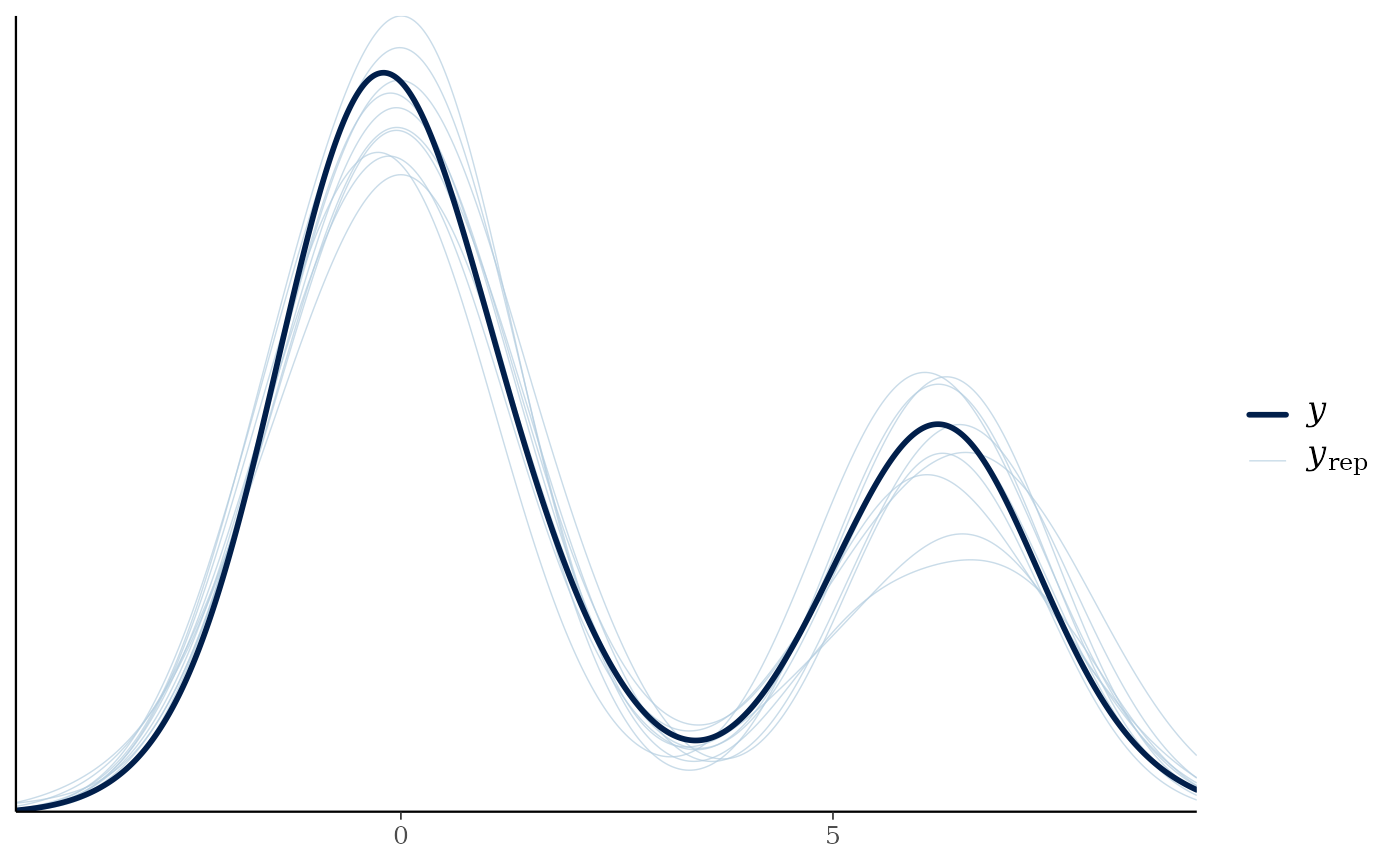
pp_check(fit4)
#> Using 10 posterior draws for ppc type 'dens_overlay' by default.
## predict the mixing proportions
fit4 <- brm(bf(y ~ x + z, theta2 ~ x),
dat, family = mix, prior = prior,
init = 0, chains = 2)
#> Compiling Stan program...
#> Start sampling
#>
#> SAMPLING FOR MODEL 'anon_model' NOW (CHAIN 1).
#> Chain 1:
#> Chain 1: Gradient evaluation took 0.000235 seconds
#> Chain 1: 1000 transitions using 10 leapfrog steps per transition would take 2.35 seconds.
#> Chain 1: Adjust your expectations accordingly!
#> Chain 1:
#> Chain 1:
#> Chain 1: Iteration: 1 / 2000 [ 0%] (Warmup)
#> Chain 1: Iteration: 200 / 2000 [ 10%] (Warmup)
#> Chain 1: Iteration: 400 / 2000 [ 20%] (Warmup)
#> Chain 1: Iteration: 600 / 2000 [ 30%] (Warmup)
#> Chain 1: Iteration: 800 / 2000 [ 40%] (Warmup)
#> Chain 1: Iteration: 1000 / 2000 [ 50%] (Warmup)
#> Chain 1: Iteration: 1001 / 2000 [ 50%] (Sampling)
#> Chain 1: Iteration: 1200 / 2000 [ 60%] (Sampling)
#> Chain 1: Iteration: 1400 / 2000 [ 70%] (Sampling)
#> Chain 1: Iteration: 1600 / 2000 [ 80%] (Sampling)
#> Chain 1: Iteration: 1800 / 2000 [ 90%] (Sampling)
#> Chain 1: Iteration: 2000 / 2000 [100%] (Sampling)
#> Chain 1:
#> Chain 1: Elapsed Time: 2.058 seconds (Warm-up)
#> Chain 1: 1.539 seconds (Sampling)
#> Chain 1: 3.597 seconds (Total)
#> Chain 1:
#>
#> SAMPLING FOR MODEL 'anon_model' NOW (CHAIN 2).
#> Chain 2:
#> Chain 2: Gradient evaluation took 0.000195 seconds
#> Chain 2: 1000 transitions using 10 leapfrog steps per transition would take 1.95 seconds.
#> Chain 2: Adjust your expectations accordingly!
#> Chain 2:
#> Chain 2:
#> Chain 2: Iteration: 1 / 2000 [ 0%] (Warmup)
#> Chain 2: Iteration: 200 / 2000 [ 10%] (Warmup)
#> Chain 2: Iteration: 400 / 2000 [ 20%] (Warmup)
#> Chain 2: Iteration: 600 / 2000 [ 30%] (Warmup)
#> Chain 2: Iteration: 800 / 2000 [ 40%] (Warmup)
#> Chain 2: Iteration: 1000 / 2000 [ 50%] (Warmup)
#> Chain 2: Iteration: 1001 / 2000 [ 50%] (Sampling)
#> Chain 2: Iteration: 1200 / 2000 [ 60%] (Sampling)
#> Chain 2: Iteration: 1400 / 2000 [ 70%] (Sampling)
#> Chain 2: Iteration: 1600 / 2000 [ 80%] (Sampling)
#> Chain 2: Iteration: 1800 / 2000 [ 90%] (Sampling)
#> Chain 2: Iteration: 2000 / 2000 [100%] (Sampling)
#> Chain 2:
#> Chain 2: Elapsed Time: 2.131 seconds (Warm-up)
#> Chain 2: 1.555 seconds (Sampling)
#> Chain 2: 3.686 seconds (Total)
#> Chain 2:
summary(fit4)
#> Family: mixture(gaussian, gaussian)
#> Links: mu1 = identity; mu2 = identity; theta2 = identity
#> Formula: y ~ x + z
#> theta2 ~ x
#> Data: dat (Number of observations: 300)
#> Draws: 2 chains, each with iter = 2000; warmup = 1000; thin = 1;
#> total post-warmup draws = 2000
#>
#> Regression Coefficients:
#> Estimate Est.Error l-95% CI u-95% CI Rhat Bulk_ESS Tail_ESS
#> mu1_Intercept 0.05 0.12 -0.18 0.27 1.00 2524 1687
#> mu2_Intercept 6.22 0.13 5.96 6.47 1.00 3067 1692
#> theta2_Intercept -0.72 0.12 -0.97 -0.48 1.00 3371 1547
#> mu1_x 0.06 0.07 -0.08 0.19 1.00 3774 1369
#> mu1_z -0.17 0.16 -0.47 0.14 1.00 3222 1349
#> mu2_x -0.08 0.11 -0.29 0.13 1.00 3453 1256
#> mu2_z -0.10 0.19 -0.48 0.28 1.00 3733 1413
#> theta2_x -0.11 0.12 -0.34 0.12 1.00 4154 1470
#>
#> Further Distributional Parameters:
#> Estimate Est.Error l-95% CI u-95% CI Rhat Bulk_ESS Tail_ESS
#> sigma1 1.04 0.05 0.95 1.15 1.00 3340 1561
#> sigma2 0.93 0.08 0.79 1.11 1.00 3589 1244
#>
#> Draws were sampled using sampling(NUTS). For each parameter, Bulk_ESS
#> and Tail_ESS are effective sample size measures, and Rhat is the potential
#> scale reduction factor on split chains (at convergence, Rhat = 1).
pp_check(fit4)
#> Using 10 posterior draws for ppc type 'dens_overlay' by default.
 ## predict all mixing proportions without a reference category
## (requires informative priors on the theta parameters)
mix_na <- mixture(gaussian, gaussian, refcat = NA)
#> Setting order = 'mu' for mixtures of the same family.
theta_prior <- c(prior, prior(normal(0, 1), Intercept, dpar = theta1),
prior(normal(0, 1), Intercept, dpar = theta2))
fit5 <- brm(bf(y ~ x + z, theta1 ~ x, theta2 ~ x),
dat, family = mix_na, prior = theta_prior,
init = 0, chains = 2)
#> Compiling Stan program...
#> Start sampling
#>
#> SAMPLING FOR MODEL 'anon_model' NOW (CHAIN 1).
#> Chain 1:
#> Chain 1: Gradient evaluation took 0.000244 seconds
#> Chain 1: 1000 transitions using 10 leapfrog steps per transition would take 2.44 seconds.
#> Chain 1: Adjust your expectations accordingly!
#> Chain 1:
#> Chain 1:
#> Chain 1: Iteration: 1 / 2000 [ 0%] (Warmup)
#> Chain 1: Iteration: 200 / 2000 [ 10%] (Warmup)
#> Chain 1: Iteration: 400 / 2000 [ 20%] (Warmup)
#> Chain 1: Iteration: 600 / 2000 [ 30%] (Warmup)
#> Chain 1: Iteration: 800 / 2000 [ 40%] (Warmup)
#> Chain 1: Iteration: 1000 / 2000 [ 50%] (Warmup)
#> Chain 1: Iteration: 1001 / 2000 [ 50%] (Sampling)
#> Chain 1: Iteration: 1200 / 2000 [ 60%] (Sampling)
#> Chain 1: Iteration: 1400 / 2000 [ 70%] (Sampling)
#> Chain 1: Iteration: 1600 / 2000 [ 80%] (Sampling)
#> Chain 1: Iteration: 1800 / 2000 [ 90%] (Sampling)
#> Chain 1: Iteration: 2000 / 2000 [100%] (Sampling)
#> Chain 1:
#> Chain 1: Elapsed Time: 164.188 seconds (Warm-up)
#> Chain 1: 193.818 seconds (Sampling)
#> Chain 1: 358.006 seconds (Total)
#> Chain 1:
#>
#> SAMPLING FOR MODEL 'anon_model' NOW (CHAIN 2).
#> Chain 2:
#> Chain 2: Gradient evaluation took 0.000208 seconds
#> Chain 2: 1000 transitions using 10 leapfrog steps per transition would take 2.08 seconds.
#> Chain 2: Adjust your expectations accordingly!
#> Chain 2:
#> Chain 2:
#> Chain 2: Iteration: 1 / 2000 [ 0%] (Warmup)
#> Chain 2: Iteration: 200 / 2000 [ 10%] (Warmup)
#> Chain 2: Iteration: 400 / 2000 [ 20%] (Warmup)
#> Chain 2: Iteration: 600 / 2000 [ 30%] (Warmup)
#> Chain 2: Iteration: 800 / 2000 [ 40%] (Warmup)
#> Chain 2: Iteration: 1000 / 2000 [ 50%] (Warmup)
#> Chain 2: Iteration: 1001 / 2000 [ 50%] (Sampling)
#> Chain 2: Iteration: 1200 / 2000 [ 60%] (Sampling)
#> Chain 2: Iteration: 1400 / 2000 [ 70%] (Sampling)
#> Chain 2: Iteration: 1600 / 2000 [ 80%] (Sampling)
#> Chain 2: Iteration: 1800 / 2000 [ 90%] (Sampling)
#> Chain 2: Iteration: 2000 / 2000 [100%] (Sampling)
#> Chain 2:
#> Chain 2: Elapsed Time: 162.17 seconds (Warm-up)
#> Chain 2: 198.394 seconds (Sampling)
#> Chain 2: 360.564 seconds (Total)
#> Chain 2:
#> Warning: There were 222 divergent transitions after warmup. See
#> https://mc-stan.org/misc/warnings.html#divergent-transitions-after-warmup
#> to find out why this is a problem and how to eliminate them.
#> Warning: There were 1776 transitions after warmup that exceeded the maximum treedepth. Increase max_treedepth above 10. See
#> https://mc-stan.org/misc/warnings.html#maximum-treedepth-exceeded
#> Warning: Examine the pairs() plot to diagnose sampling problems
#> Warning: Bulk Effective Samples Size (ESS) is too low, indicating posterior means and medians may be unreliable.
#> Running the chains for more iterations may help. See
#> https://mc-stan.org/misc/warnings.html#bulk-ess
#> Warning: Tail Effective Samples Size (ESS) is too low, indicating posterior variances and tail quantiles may be unreliable.
#> Running the chains for more iterations may help. See
#> https://mc-stan.org/misc/warnings.html#tail-ess
summary(fit5)
#> Warning: There were 222 divergent transitions after warmup. Increasing adapt_delta above 0.8 may help. See http://mc-stan.org/misc/warnings.html#divergent-transitions-after-warmup
#> Family: mixture(gaussian, gaussian)
#> Links: mu1 = identity; mu2 = identity; theta1 = identity; theta2 = identity
#> Formula: y ~ x + z
#> theta1 ~ x
#> theta2 ~ x
#> Data: dat (Number of observations: 300)
#> Draws: 2 chains, each with iter = 2000; warmup = 1000; thin = 1;
#> total post-warmup draws = 2000
#>
#> Regression Coefficients:
#> Estimate Est.Error l-95% CI u-95% CI Rhat Bulk_ESS Tail_ESS
#> mu1_Intercept 0.06 0.12 -0.16 0.29 1.03 50 165
#> mu2_Intercept 6.21 0.12 5.95 6.45 1.01 88 231
#> theta1_Intercept 1.38 6.62 -10.98 11.58 1.04 32 75
#> theta2_Intercept 0.67 6.62 -11.78 10.88 1.04 32 75
#> mu1_x 0.07 0.07 -0.07 0.21 1.01 105 146
#> mu1_z -0.17 0.15 -0.48 0.12 1.01 97 122
#> mu2_x -0.08 0.10 -0.28 0.12 1.01 83 258
#> mu2_z -0.10 0.18 -0.43 0.26 1.02 91 206
#> theta1_x 16.64 117.47 -202.95 205.84 1.05 32 90
#> theta2_x 16.53 117.48 -202.88 205.84 1.05 32 93
#>
#> Further Distributional Parameters:
#> Estimate Est.Error l-95% CI u-95% CI Rhat Bulk_ESS Tail_ESS
#> sigma1 1.04 0.05 0.95 1.14 1.01 98 212
#> sigma2 0.93 0.09 0.80 1.12 1.02 72 73
#>
#> Draws were sampled using sampling(NUTS). For each parameter, Bulk_ESS
#> and Tail_ESS are effective sample size measures, and Rhat is the potential
#> scale reduction factor on split chains (at convergence, Rhat = 1).
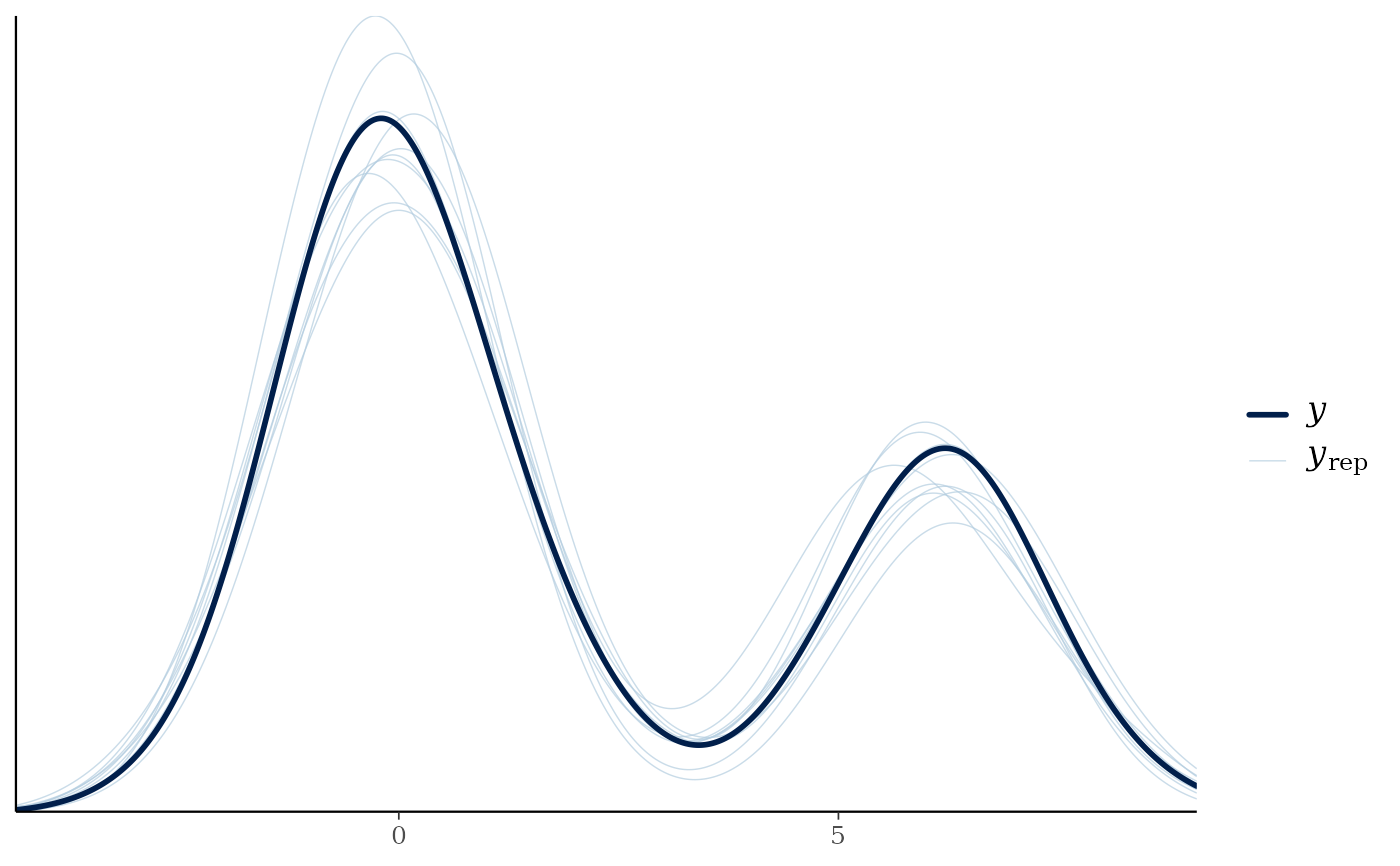
pp_check(fit5)
#> Using 10 posterior draws for ppc type 'dens_overlay' by default.
## predict all mixing proportions without a reference category
## (requires informative priors on the theta parameters)
mix_na <- mixture(gaussian, gaussian, refcat = NA)
#> Setting order = 'mu' for mixtures of the same family.
theta_prior <- c(prior, prior(normal(0, 1), Intercept, dpar = theta1),
prior(normal(0, 1), Intercept, dpar = theta2))
fit5 <- brm(bf(y ~ x + z, theta1 ~ x, theta2 ~ x),
dat, family = mix_na, prior = theta_prior,
init = 0, chains = 2)
#> Compiling Stan program...
#> Start sampling
#>
#> SAMPLING FOR MODEL 'anon_model' NOW (CHAIN 1).
#> Chain 1:
#> Chain 1: Gradient evaluation took 0.000244 seconds
#> Chain 1: 1000 transitions using 10 leapfrog steps per transition would take 2.44 seconds.
#> Chain 1: Adjust your expectations accordingly!
#> Chain 1:
#> Chain 1:
#> Chain 1: Iteration: 1 / 2000 [ 0%] (Warmup)
#> Chain 1: Iteration: 200 / 2000 [ 10%] (Warmup)
#> Chain 1: Iteration: 400 / 2000 [ 20%] (Warmup)
#> Chain 1: Iteration: 600 / 2000 [ 30%] (Warmup)
#> Chain 1: Iteration: 800 / 2000 [ 40%] (Warmup)
#> Chain 1: Iteration: 1000 / 2000 [ 50%] (Warmup)
#> Chain 1: Iteration: 1001 / 2000 [ 50%] (Sampling)
#> Chain 1: Iteration: 1200 / 2000 [ 60%] (Sampling)
#> Chain 1: Iteration: 1400 / 2000 [ 70%] (Sampling)
#> Chain 1: Iteration: 1600 / 2000 [ 80%] (Sampling)
#> Chain 1: Iteration: 1800 / 2000 [ 90%] (Sampling)
#> Chain 1: Iteration: 2000 / 2000 [100%] (Sampling)
#> Chain 1:
#> Chain 1: Elapsed Time: 164.188 seconds (Warm-up)
#> Chain 1: 193.818 seconds (Sampling)
#> Chain 1: 358.006 seconds (Total)
#> Chain 1:
#>
#> SAMPLING FOR MODEL 'anon_model' NOW (CHAIN 2).
#> Chain 2:
#> Chain 2: Gradient evaluation took 0.000208 seconds
#> Chain 2: 1000 transitions using 10 leapfrog steps per transition would take 2.08 seconds.
#> Chain 2: Adjust your expectations accordingly!
#> Chain 2:
#> Chain 2:
#> Chain 2: Iteration: 1 / 2000 [ 0%] (Warmup)
#> Chain 2: Iteration: 200 / 2000 [ 10%] (Warmup)
#> Chain 2: Iteration: 400 / 2000 [ 20%] (Warmup)
#> Chain 2: Iteration: 600 / 2000 [ 30%] (Warmup)
#> Chain 2: Iteration: 800 / 2000 [ 40%] (Warmup)
#> Chain 2: Iteration: 1000 / 2000 [ 50%] (Warmup)
#> Chain 2: Iteration: 1001 / 2000 [ 50%] (Sampling)
#> Chain 2: Iteration: 1200 / 2000 [ 60%] (Sampling)
#> Chain 2: Iteration: 1400 / 2000 [ 70%] (Sampling)
#> Chain 2: Iteration: 1600 / 2000 [ 80%] (Sampling)
#> Chain 2: Iteration: 1800 / 2000 [ 90%] (Sampling)
#> Chain 2: Iteration: 2000 / 2000 [100%] (Sampling)
#> Chain 2:
#> Chain 2: Elapsed Time: 162.17 seconds (Warm-up)
#> Chain 2: 198.394 seconds (Sampling)
#> Chain 2: 360.564 seconds (Total)
#> Chain 2:
#> Warning: There were 222 divergent transitions after warmup. See
#> https://mc-stan.org/misc/warnings.html#divergent-transitions-after-warmup
#> to find out why this is a problem and how to eliminate them.
#> Warning: There were 1776 transitions after warmup that exceeded the maximum treedepth. Increase max_treedepth above 10. See
#> https://mc-stan.org/misc/warnings.html#maximum-treedepth-exceeded
#> Warning: Examine the pairs() plot to diagnose sampling problems
#> Warning: Bulk Effective Samples Size (ESS) is too low, indicating posterior means and medians may be unreliable.
#> Running the chains for more iterations may help. See
#> https://mc-stan.org/misc/warnings.html#bulk-ess
#> Warning: Tail Effective Samples Size (ESS) is too low, indicating posterior variances and tail quantiles may be unreliable.
#> Running the chains for more iterations may help. See
#> https://mc-stan.org/misc/warnings.html#tail-ess
summary(fit5)
#> Warning: There were 222 divergent transitions after warmup. Increasing adapt_delta above 0.8 may help. See http://mc-stan.org/misc/warnings.html#divergent-transitions-after-warmup
#> Family: mixture(gaussian, gaussian)
#> Links: mu1 = identity; mu2 = identity; theta1 = identity; theta2 = identity
#> Formula: y ~ x + z
#> theta1 ~ x
#> theta2 ~ x
#> Data: dat (Number of observations: 300)
#> Draws: 2 chains, each with iter = 2000; warmup = 1000; thin = 1;
#> total post-warmup draws = 2000
#>
#> Regression Coefficients:
#> Estimate Est.Error l-95% CI u-95% CI Rhat Bulk_ESS Tail_ESS
#> mu1_Intercept 0.06 0.12 -0.16 0.29 1.03 50 165
#> mu2_Intercept 6.21 0.12 5.95 6.45 1.01 88 231
#> theta1_Intercept 1.38 6.62 -10.98 11.58 1.04 32 75
#> theta2_Intercept 0.67 6.62 -11.78 10.88 1.04 32 75
#> mu1_x 0.07 0.07 -0.07 0.21 1.01 105 146
#> mu1_z -0.17 0.15 -0.48 0.12 1.01 97 122
#> mu2_x -0.08 0.10 -0.28 0.12 1.01 83 258
#> mu2_z -0.10 0.18 -0.43 0.26 1.02 91 206
#> theta1_x 16.64 117.47 -202.95 205.84 1.05 32 90
#> theta2_x 16.53 117.48 -202.88 205.84 1.05 32 93
#>
#> Further Distributional Parameters:
#> Estimate Est.Error l-95% CI u-95% CI Rhat Bulk_ESS Tail_ESS
#> sigma1 1.04 0.05 0.95 1.14 1.01 98 212
#> sigma2 0.93 0.09 0.80 1.12 1.02 72 73
#>
#> Draws were sampled using sampling(NUTS). For each parameter, Bulk_ESS
#> and Tail_ESS are effective sample size measures, and Rhat is the potential
#> scale reduction factor on split chains (at convergence, Rhat = 1).
pp_check(fit5)
#> Using 10 posterior draws for ppc type 'dens_overlay' by default.
 ## compare model fit
loo(fit1, fit2, fit3, fit4)
#> Output of model 'fit1':
#>
#> Computed from 2000 by 300 log-likelihood matrix.
#>
#> Estimate SE
#> elpd_loo -721.1 10.0
#> p_loo 61.6 3.7
#> looic 1442.1 19.9
#> ------
#> MCSE of elpd_loo is 5.0.
#> MCSE and ESS estimates assume MCMC draws (r_eff in [0.0, 1.7]).
#>
#> All Pareto k estimates are good (k < 0.7).
#> See help('pareto-k-diagnostic') for details.
#>
#> Output of model 'fit2':
#>
#> Computed from 2000 by 300 log-likelihood matrix.
#>
#> Estimate SE
#> elpd_loo -721.1 17.0
#> p_loo 71.6 5.8
#> looic 1442.1 33.9
#> ------
#> MCSE of elpd_loo is 4.7.
#> MCSE and ESS estimates assume MCMC draws (r_eff in [0.0, 1.5]).
#>
#> All Pareto k estimates are good (k < 0.7).
#> See help('pareto-k-diagnostic') for details.
#>
#> Output of model 'fit3':
#>
#> Computed from 2000 by 300 log-likelihood matrix.
#>
#> Estimate SE
#> elpd_loo -683.6 11.1
#> p_loo 7.6 0.6
#> looic 1367.2 22.2
#> ------
#> MCSE of elpd_loo is 0.1.
#> MCSE and ESS estimates assume MCMC draws (r_eff in [0.9, 1.8]).
#>
#> All Pareto k estimates are good (k < 0.7).
#> See help('pareto-k-diagnostic') for details.
#>
#> Output of model 'fit4':
#>
#> Computed from 2000 by 300 log-likelihood matrix.
#>
#> Estimate SE
#> elpd_loo -620.7 13.9
#> p_loo 10.5 1.1
#> looic 1241.4 27.7
#> ------
#> MCSE of elpd_loo is 0.1.
#> MCSE and ESS estimates assume MCMC draws (r_eff in [0.9, 2.5]).
#>
#> All Pareto k estimates are good (k < 0.7).
#> See help('pareto-k-diagnostic') for details.
#>
#> Model comparisons:
#> model elpd_diff se_diff p_worse diag_diff diag_elpd
#> fit4 0.0 0.0 NA
#> fit3 -62.9 9.9 1.00
#> fit1 -100.4 5.9 1.00
#> fit2 -100.4 10.1 1.00
# }
## compare model fit
loo(fit1, fit2, fit3, fit4)
#> Output of model 'fit1':
#>
#> Computed from 2000 by 300 log-likelihood matrix.
#>
#> Estimate SE
#> elpd_loo -721.1 10.0
#> p_loo 61.6 3.7
#> looic 1442.1 19.9
#> ------
#> MCSE of elpd_loo is 5.0.
#> MCSE and ESS estimates assume MCMC draws (r_eff in [0.0, 1.7]).
#>
#> All Pareto k estimates are good (k < 0.7).
#> See help('pareto-k-diagnostic') for details.
#>
#> Output of model 'fit2':
#>
#> Computed from 2000 by 300 log-likelihood matrix.
#>
#> Estimate SE
#> elpd_loo -721.1 17.0
#> p_loo 71.6 5.8
#> looic 1442.1 33.9
#> ------
#> MCSE of elpd_loo is 4.7.
#> MCSE and ESS estimates assume MCMC draws (r_eff in [0.0, 1.5]).
#>
#> All Pareto k estimates are good (k < 0.7).
#> See help('pareto-k-diagnostic') for details.
#>
#> Output of model 'fit3':
#>
#> Computed from 2000 by 300 log-likelihood matrix.
#>
#> Estimate SE
#> elpd_loo -683.6 11.1
#> p_loo 7.6 0.6
#> looic 1367.2 22.2
#> ------
#> MCSE of elpd_loo is 0.1.
#> MCSE and ESS estimates assume MCMC draws (r_eff in [0.9, 1.8]).
#>
#> All Pareto k estimates are good (k < 0.7).
#> See help('pareto-k-diagnostic') for details.
#>
#> Output of model 'fit4':
#>
#> Computed from 2000 by 300 log-likelihood matrix.
#>
#> Estimate SE
#> elpd_loo -620.7 13.9
#> p_loo 10.5 1.1
#> looic 1241.4 27.7
#> ------
#> MCSE of elpd_loo is 0.1.
#> MCSE and ESS estimates assume MCMC draws (r_eff in [0.9, 2.5]).
#>
#> All Pareto k estimates are good (k < 0.7).
#> See help('pareto-k-diagnostic') for details.
#>
#> Model comparisons:
#> model elpd_diff se_diff p_worse diag_diff diag_elpd
#> fit4 0.0 0.0 NA
#> fit3 -62.9 9.9 1.00
#> fit1 -100.4 5.9 1.00
#> fit2 -100.4 10.1 1.00
# }