Expected Values of the Posterior Predictive Distribution

This method is an alias of posterior_epred.brmsfit with additional arguments for obtaining summaries of the computed draws.

Usage

# S3 method for class 'brmsfit'
fitted(
  object,
  newdata = NULL,
  re_formula = NULL,
  scale = c("response", "linear"),
  resp = NULL,
  dpar = NULL,
  nlpar = NULL,
  ndraws = NULL,
  draw_ids = NULL,
  sort = FALSE,
  summary = TRUE,
  robust = FALSE,
  probs = c(0.025, 0.975),
  ...
)

Arguments

object: An object of class brmsfit.
newdata: An optional data.frame for which to evaluate predictions. If NULL (default), the original data of the model is used. NA values within factors (excluding grouping variables) are interpreted as if all dummy variables of this factor are zero. This allows, for instance, to make predictions of the grand mean when using sum coding. NA values within grouping variables are treated as a new level.
re_formula: formula containing group-level effects to be considered in the prediction. If NULL (default), include all group-level effects; if NA or ~0, include no group-level effects.
scale: Either "response" or "linear". If "response", results are returned on the scale of the response variable. If "linear", results are returned on the scale of the linear predictor term, that is without applying the inverse link function or other transformations.
resp: Optional names of response variables. If specified, predictions are performed only for the specified response variables.
dpar: Optional name of a predicted distributional parameter. If specified, expected predictions of this parameters are returned.
nlpar: Optional name of a predicted non-linear parameter. If specified, expected predictions of this parameters are returned.
ndraws: Positive integer indicating how many posterior draws should be used. If NULL (the default) all draws are used. Ignored if draw_ids is not NULL.
draw_ids: An integer vector specifying the posterior draws to be used. If NULL (the default), all draws are used.
sort: Logical. Only relevant for time series models. Indicating whether to return predicted values in the original order (FALSE; default) or in the order of the time series (TRUE).
summary: Should summary statistics be returned instead of the raw values? Default is TRUE..
robust: If FALSE (the default) the mean is used as the measure of central tendency and the standard deviation as the measure of variability. If TRUE, the median and the median absolute deviation (MAD) are applied instead. Only used if summary is TRUE.
probs: The percentiles to be computed by the quantile function. Only used if summary is TRUE.
...: Further arguments passed to prepare_predictions that control several aspects of data validation and prediction.

Value

An array of predicted mean response values. If summary = FALSE the output resembles those of posterior_epred.brmsfit.

If summary = TRUE the output depends on the family: For categorical and ordinal families, the output is an N x E x C array, where N is the number of observations, E is the number of summary statistics, and C is the number of categories. For all other families, the output is an N x E matrix. The number of summary statistics E is equal to 2 + length(probs): The Estimate column contains point estimates (either mean or median depending on argument robust), while the Est.Error column contains uncertainty estimates (either standard deviation or median absolute deviation depending on argument robust). The remaining columns starting with Q contain quantile estimates as specified via argument probs.

In multivariate models, an additional dimension is added to the output which indexes along the different response variables.

Examples

# \dontrun{
## fit a model
fit <- brm(rating ~ treat + period + carry + (1|subject),
           data = inhaler)
#> Compiling Stan program...
#> Start sampling
#> 
#> SAMPLING FOR MODEL 'anon_model' NOW (CHAIN 1).
#> Chain 1: 
#> Chain 1: Gradient evaluation took 5.4e-05 seconds
#> Chain 1: 1000 transitions using 10 leapfrog steps per transition would take 0.54 seconds.
#> Chain 1: Adjust your expectations accordingly!
#> Chain 1: 
#> Chain 1: 
#> Chain 1: Iteration:    1 / 2000 [  0%]  (Warmup)
#> Chain 1: Iteration:  200 / 2000 [ 10%]  (Warmup)
#> Chain 1: Iteration:  400 / 2000 [ 20%]  (Warmup)
#> Chain 1: Iteration:  600 / 2000 [ 30%]  (Warmup)
#> Chain 1: Iteration:  800 / 2000 [ 40%]  (Warmup)
#> Chain 1: Iteration: 1000 / 2000 [ 50%]  (Warmup)
#> Chain 1: Iteration: 1001 / 2000 [ 50%]  (Sampling)
#> Chain 1: Iteration: 1200 / 2000 [ 60%]  (Sampling)
#> Chain 1: Iteration: 1400 / 2000 [ 70%]  (Sampling)
#> Chain 1: Iteration: 1600 / 2000 [ 80%]  (Sampling)
#> Chain 1: Iteration: 1800 / 2000 [ 90%]  (Sampling)
#> Chain 1: Iteration: 2000 / 2000 [100%]  (Sampling)
#> Chain 1: 
#> Chain 1:  Elapsed Time: 1.609 seconds (Warm-up)
#> Chain 1:                0.774 seconds (Sampling)
#> Chain 1:                2.383 seconds (Total)
#> Chain 1: 
#> 
#> SAMPLING FOR MODEL 'anon_model' NOW (CHAIN 2).
#> Chain 2: 
#> Chain 2: Gradient evaluation took 4.5e-05 seconds
#> Chain 2: 1000 transitions using 10 leapfrog steps per transition would take 0.45 seconds.
#> Chain 2: Adjust your expectations accordingly!
#> Chain 2: 
#> Chain 2: 
#> Chain 2: Iteration:    1 / 2000 [  0%]  (Warmup)
#> Chain 2: Iteration:  200 / 2000 [ 10%]  (Warmup)
#> Chain 2: Iteration:  400 / 2000 [ 20%]  (Warmup)
#> Chain 2: Iteration:  600 / 2000 [ 30%]  (Warmup)
#> Chain 2: Iteration:  800 / 2000 [ 40%]  (Warmup)
#> Chain 2: Iteration: 1000 / 2000 [ 50%]  (Warmup)
#> Chain 2: Iteration: 1001 / 2000 [ 50%]  (Sampling)
#> Chain 2: Iteration: 1200 / 2000 [ 60%]  (Sampling)
#> Chain 2: Iteration: 1400 / 2000 [ 70%]  (Sampling)
#> Chain 2: Iteration: 1600 / 2000 [ 80%]  (Sampling)
#> Chain 2: Iteration: 1800 / 2000 [ 90%]  (Sampling)
#> Chain 2: Iteration: 2000 / 2000 [100%]  (Sampling)
#> Chain 2: 
#> Chain 2:  Elapsed Time: 1.563 seconds (Warm-up)
#> Chain 2:                0.776 seconds (Sampling)
#> Chain 2:                2.339 seconds (Total)
#> Chain 2: 
#> 
#> SAMPLING FOR MODEL 'anon_model' NOW (CHAIN 3).
#> Chain 3: 
#> Chain 3: Gradient evaluation took 6.8e-05 seconds
#> Chain 3: 1000 transitions using 10 leapfrog steps per transition would take 0.68 seconds.
#> Chain 3: Adjust your expectations accordingly!
#> Chain 3: 
#> Chain 3: 
#> Chain 3: Iteration:    1 / 2000 [  0%]  (Warmup)
#> Chain 3: Iteration:  200 / 2000 [ 10%]  (Warmup)
#> Chain 3: Iteration:  400 / 2000 [ 20%]  (Warmup)
#> Chain 3: Iteration:  600 / 2000 [ 30%]  (Warmup)
#> Chain 3: Iteration:  800 / 2000 [ 40%]  (Warmup)
#> Chain 3: Iteration: 1000 / 2000 [ 50%]  (Warmup)
#> Chain 3: Iteration: 1001 / 2000 [ 50%]  (Sampling)
#> Chain 3: Iteration: 1200 / 2000 [ 60%]  (Sampling)
#> Chain 3: Iteration: 1400 / 2000 [ 70%]  (Sampling)
#> Chain 3: Iteration: 1600 / 2000 [ 80%]  (Sampling)
#> Chain 3: Iteration: 1800 / 2000 [ 90%]  (Sampling)
#> Chain 3: Iteration: 2000 / 2000 [100%]  (Sampling)
#> Chain 3: 
#> Chain 3:  Elapsed Time: 1.621 seconds (Warm-up)
#> Chain 3:                0.775 seconds (Sampling)
#> Chain 3:                2.396 seconds (Total)
#> Chain 3: 
#> 
#> SAMPLING FOR MODEL 'anon_model' NOW (CHAIN 4).
#> Chain 4: 
#> Chain 4: Gradient evaluation took 4.5e-05 seconds
#> Chain 4: 1000 transitions using 10 leapfrog steps per transition would take 0.45 seconds.
#> Chain 4: Adjust your expectations accordingly!
#> Chain 4: 
#> Chain 4: 
#> Chain 4: Iteration:    1 / 2000 [  0%]  (Warmup)
#> Chain 4: Iteration:  200 / 2000 [ 10%]  (Warmup)
#> Chain 4: Iteration:  400 / 2000 [ 20%]  (Warmup)
#> Chain 4: Iteration:  600 / 2000 [ 30%]  (Warmup)
#> Chain 4: Iteration:  800 / 2000 [ 40%]  (Warmup)
#> Chain 4: Iteration: 1000 / 2000 [ 50%]  (Warmup)
#> Chain 4: Iteration: 1001 / 2000 [ 50%]  (Sampling)
#> Chain 4: Iteration: 1200 / 2000 [ 60%]  (Sampling)
#> Chain 4: Iteration: 1400 / 2000 [ 70%]  (Sampling)
#> Chain 4: Iteration: 1600 / 2000 [ 80%]  (Sampling)
#> Chain 4: Iteration: 1800 / 2000 [ 90%]  (Sampling)
#> Chain 4: Iteration: 2000 / 2000 [100%]  (Sampling)
#> Chain 4: 
#> Chain 4:  Elapsed Time: 1.706 seconds (Warm-up)
#> Chain 4:                0.774 seconds (Sampling)
#> Chain 4:                2.48 seconds (Total)
#> Chain 4: 

## compute expected predictions
fitted_values <- fitted(fit)
head(fitted_values)
#>      Estimate Est.Error      Q2.5    Q97.5
#> [1,] 1.203823 0.2146653 0.7774631 1.617767
#> [2,] 1.204475 0.2131137 0.7750120 1.627070
#> [3,] 1.198250 0.2166810 0.7412610 1.602561
#> [4,] 1.199921 0.2209145 0.7452845 1.627845
#> [5,] 1.200266 0.2116506 0.7595375 1.605907
#> [6,] 1.205254 0.2217596 0.7573821 1.620766

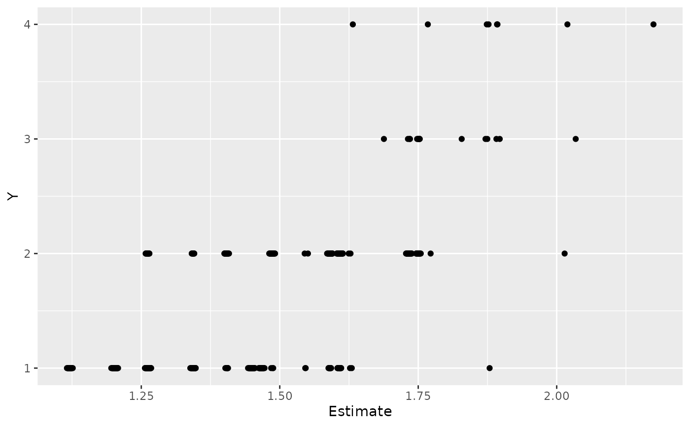
## plot expected predictions against actual response
dat <- as.data.frame(cbind(Y = standata(fit)$Y, fitted_values))
ggplot(dat) + geom_point(aes(x = Estimate, y = Y))

# }

Expected Values of the Posterior Predictive Distribution

Usage

Arguments

Value

See also

Examples