Running brms models with within-chain parallelization

Introduction

Full Bayesian inference is a computationally very demanding task and often we wish to run our models faster in shorter walltime. With modern computers we nowadays have multiple processors available on a given machine such that the use of running the inference in parallel will shorten the overall walltime. While between-chain parallelization is straightforward by merely launching multiple chains at the same time, the use of within-chain parallelization is more complicated in various ways. This vignette aims to introduce the user to within-chain parallelization with brms, since its efficient use depends on various aspects specific to the users model.

Quick summary

Assuming you have a brms model which you wish to evaluate faster by using more cores per chain, for example:

fit_serial <- brm(
  count ~ zAge + zBase * Trt + (1|patient),
  data = epilepsy, family = poisson(),
  chains = 4, cores = 4, backend = "cmdstanr"
)

Then you can simply add threading support to an existing model with the update mechanism as follows, provided your stan version is at least 2.26 (whether using rstan or cmdstan):

fit_parallel <- update(
  fit_serial, chains = 2, cores = 2,
  backend = "cmdstanr", threads = threading(2)
)

The example above assumes that 4 cores are available which are best used without within-chain parallelization by running 4 chains in parallel. When using within chain parallelization it is still advisable to use just as many threads in total as you have CPU cores. It’s thus sensible in this case to reduce the number of chains running in parallel to just 2, but allow each chain to use 2 threads. Obviously this will reduce the number of iterations in the posterior here as we assumed a fixed amount of 4 cores.

Only apply within-chain parallelization to large problems which take more than a few minutes at least to calculate. The epilepsy example above is actually too small to gain in speed (just a few seconds per chain on this machine).
Within-chain parallelization is less efficient than between-chain parallelization. So only use within-chain parallelism if more CPUs can be used to run the entire analysis.
Due to details of the model and data-set, speedups with more cores can be very limited. Not every model amends to within-chain parallelization and an empirical evaluation is in some cases advisable.
Enabling threading usually slows down any model to some extent and this slowdown must be offset by sufficient cores per chain in order to really gain in execution speed.
Doubling the execution speed with few cores is a lot easier than obtaining larger speedups with even more cores.
Models with computationally expensive likelihoods are easier to parallelize than less expensive likelihoods. For example, the Poisson distribution involves expensive \(\log\Gamma\) functions whereas the normal likelihood is very cheap to calculate in comparison.
Models with many parameters (e.g., multilevel models) carry a large overhead when running in parallel.
With a larger overhead of the model, the likelihood must be sufficiently expensive such that the relative computational cost of likelihood to parallelization overhead is favorable.
Avoid using hyper-threading, that is, only use as many threads as you have physical cores available.
Ensure that the data is randomly sorted such that consecutive subsets of the data are roughly of the same computational effort.

Within-chain parallelization

The within-chain parallelization implemented in brms is based on the reduce_sum facility in Stan. The basic principle that reduce_sum uses is to split a large summation into arbitrary smaller partial sums. Due to the commutativity and associativity of the sum operation these smaller partial sums can be evaluated in any order and in parallel from one another. brms leverages reduce_sum to evaluate the log-likelihood of the model in parallel as for example

\[ \begin{aligned} l(y|\theta) &= \sum_{i=1}^N l_i(y_i| \theta) \\ &= \sum_{i=1}^{S_1} l_i(y_i| \theta) + \sum_{i=S_1+1}^N l_i(y_i| \theta). \end{aligned} \]

As a consequence, the within-chain parallelization requires mutually independent log-likelihood terms which restricts its applicability to some degree.

Furthermore, the within-chain parallelization is only applicable to the evaluation of the data likelihood while all other parts of the model, for example priors, will remain running serially. Thus, only a partial fraction of the entire Stan model will run in parallel which limits the potential speedup one may obtain. The theoretical speedup for a partially in parallel running program is described by Amdahl‘s law. For example, with 90% of the computational load running in parallel one can essentially double the execution speed with 2 cores while 8 cores may only speedup the program by at most 5x. How large the computational cost of the log-likelihood is in relation to the entire model is very dependent on the model of the user.

In practice, the speedups are even smaller than the theoretical speedups. This is caused by the additional overhead implied by forming multiple smaller sums than just one large one. For example, for each partial sum formed the entire parameter vector \(\theta\) has to be copied in memory for Stan to be able to calculate the gradient of the log-likelihood. Hence, with more partial sums, more copying is necessary as opposed to evaluating just one large sum. Whether the additional copying is indeed relevant depends on the computational cost of the log-likelihood of each term and the number of parameters. For a model with a computationally cheap normal log-likelihood, this effect is more important than for a model with a Poisson log-likelihood, and for multilevel models with many parameters more copying is needed than for simpler regression models. It may therefore be necessary to form sufficiently large partial sums to warrant an efficient parallel execution. The size of the partial sums is referred to as the grainsize, which is set to a reasonable default value. However, for some models this tuning parameter requires some attention from the user for optimal performance.

Finally, it is important to note that by default the exact size and order of the partial sums is not stable as it is adjusted to the load of the system. As a result, exact numerical reproducibility is not guaranteed by default. In order to warrant the same size and order of the partial sums, the static option must be used and set to TRUE, which uses a deterministic scheduler for the parallel work.

Example model

As a toy demonstration, we use here a multilevel Poisson model. The model is a varying intercept model with \(10^{4}\) data observation which are grouped into \(1000\) groups. Each data item has \(3\) continuous covariates. The simulation code for the fake data can be found in the appendix and it’s first \(10\) rows are:

kable(head(fake, 10), digits = 3)

g	x1	x2	x3	theta	eta	mu	y
382	0.496	0.623	0.069	-0.262	0.510	0.248	0
578	-0.748	-0.300	-0.768	-0.903	-0.032	-0.934	0
772	-1.124	-0.161	-0.882	-1.047	-0.551	-1.598	1
774	0.992	-0.593	1.007	1.578	-0.045	1.533	2
729	0.641	-1.563	-0.491	-0.291	-1.460	-1.751	0
897	-0.085	-0.531	-0.978	-1.296	-0.929	-2.226	0
110	-0.772	1.364	-0.629	-1.351	0.124	-1.227	0
248	-1.441	0.699	1.284	2.072	-1.020	1.053	1
754	-1.320	0.837	-0.137	-0.237	1.452	1.215	3
682	-1.345	-2.673	-1.628	-1.146	-0.388	-1.534	0

The brms model fitting this data is:

model_poisson <- brm(
  y ~ 1 + x1 + x2 + (1 | g),
  data = fake,
  family = poisson(),
  iter = 500, # short sampling to speedup example
  chains = 2,
  prior = prior(normal(0,1), class = b) +
    prior(constant(1), class = sd, group = g),
  backend = "cmdstanr",
  threads = threading(4),
  save_pars = save_pars(all = TRUE)
)

Here we have fixed the standard deviation of the between-group variation for the intercept to the true value of \(1\) as used in the simulation. This is to avoid unfavorable geometry of the problem allowing us to concentrate on computational aspects alone.

The Poisson likelihood is a relatively expensive likelihood due to the use of \(\log\Gamma\) function as opposed to, for example, a normal likelihood which does is by far less expensive operations. Moreover, this example is chosen in order to demonstrate parallelization overhead implied by a large number of parameters.

Managing parallelization overhead

As discussed above, the key mechanism to run Stan programs with parallelization is to split the large sum over independent log likelihood terms into arbitrary smaller partial sums. Creating more partial sums allows to increase simultaneous parallel computations in a granular way, but at the same time additional overhead is introduced through the requirement to copy the entire parameter vector for each partial sum formed along with further overhead due to splitting up a single large task into multiple smaller ones.

By default, brms will choose a sensible grainsize which defines how large a given partial sum will roughly be. The actual chunk size is automatically tuned whenever the default non-static scheduler is used, which is the recommended choice to start with. As noted before, only the static scheduler is giving fully deterministic results since the chunk size and order of partial sums will be the same during sampling.

While we expect that the default grainsize in brms is reasonably good for many models, it can improve performance if one tunes the grainsize specifically to a given model and data-set. We suggest to increase successively the number of chunks a given data set is split into with the static scheduler and run this on a single core. This way one can control the number of partial sum accurately and monitor the execution time as it increases. These experiments are run with only a single chain and very short iteration numbers as we are not interested in the statistical results, but rather aim to be able to explore the tuning parameter space of the chunk size as quickly as possible. The number of iterations needed to get reliable runtime estimates for a given chunk size will depend on many details and the easiest way to determine this is to run this benchmark with multiple number of iterations. Whenever their results match approximately, then the iteration numbers are sufficient. In order to decrease the variation between runs, we also fix the random seed, initial value and the tuning parameters of the sampler (step size and mass matrix).

Below is an example R code demonstrating such a benchmark. The utility function benchmark_threading is shown and explained in the appendix.

chunking_bench <- transform(
    data.frame(chunks = 4^(0:3)),
    grainsize = ceiling(N / chunks)
)

iter_test <- c(10, 20, 40)  # very short test runs
scaling_chunking <- benchmark_threading(
  model_poisson,
  cores = 1,
  grainsize = chunking_bench$grainsize,  # test various grainsizes
  iter = iter_test,
  static = TRUE  # with static partitioner
)

# run as reference the model *without* reduce_sum
ref <- benchmark_reference(model_poisson, iter_test)

# for additional data munging please refer to the appendix

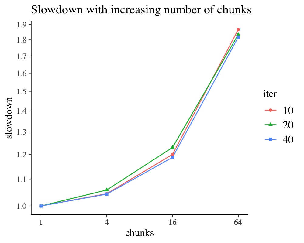
Graphically summarizing the results shows that with more than 8 chunks the overhead is about 10% and increasing further with more chunks. For models without many parameters, no such overhead should be observed. Furthermore, one can see that 25 and 50 iterations give similar results implying that 25 iterations suffice for stable runtime estimates for these (and the following) benchmarks. The overhead of up to 20% in this example with 16 chunks may seem large due to the scaling of the plot. One must not forget that when we start to use more CPU cores, the overhead is easily offset, but it limits the maximal speedup we can get. For example, some 2 units of computation become 2.4 units due to the overhead such that on 2 cores we don’t quite double the execution speed, but rather get a 1.6x increase in speed instead of a 2x speedup.

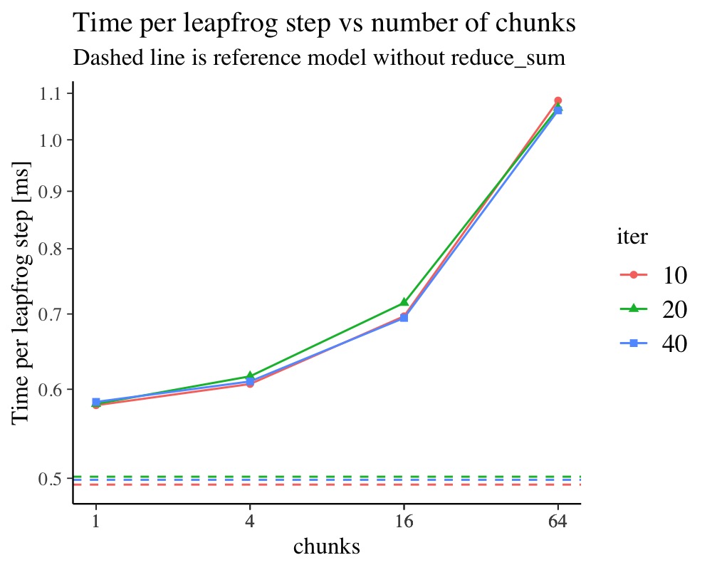
Considering in addition the time per leapfrog step of the NUTS sampler shows on an absolute scale similar information as before. The upside of this representation is that we can visualize the slowdown in relation to the program without reduce_sum. As we can see, the additional overhead due to merely enabling reduce_sum is substantial in this example. This is attributed in the specific example to the large number of random effects.

ggplot(scaling_chunking) +
    aes(chunks, slowdown, colour = iter, shape = iter) +
    geom_line() + geom_point() +
    scale_x_log10(breaks = scaling_chunking$chunks) +
    scale_y_log10(breaks=seq(0.8, 2.5, by=0.1)) +
    ggtitle("Slowdown with increasing number of chunks")

ggplot(scaling_chunking) +
    aes(chunks, 1E3 * runtime/num_leapfrog, colour = iter, shape=iter) +
    geom_line() + geom_point() +
    scale_x_log10(breaks = scaling_chunking$chunks) +
    scale_y_log10(breaks=seq(0.1, 2.0, by=0.1)) +
    geom_hline(data=ref, aes(yintercept=1E3 * runtime/num_leapfrog, colour=iter), linetype=I(2)) +
    ggtitle("Time per leapfrog step vs number of chunks",
            "Dashed line is reference model without reduce_sum") +
    ylab("Time per leapfrog step [ms]")

Parallelization speedup

In practice, we are often interested in so-called “hard-scaling” properties of the parallelization system. That is, for a fixed problem size we would like to know how much faster we can execute the Stan program with increasing number of threads. As nowadays CPUs usually run with so-called hyper-threading, it is also of interest if this technique is beneficial for Stan programs as well (spoiler alert: it’s not useful). As we have seen before, the grainsize can have an impact on the performance and is as such a tuning parameter. Below we demonstrate some exemplary R code which runs a benchmark with varying number of CPU cores and varying number of grainsizes.

num_cpu <- parallel::detectCores(logical = FALSE)
num_cpu_logical <- parallel::detectCores(logical = TRUE)
grainsize_default <- ceiling(N / (2 * num_cpu))
cores <- c(2^seq(0, floor(log2(num_cpu_logical))), num_cpu, num_cpu_logical)
cores <- sort(unique(cores))
grainsize <- c(grainsize_default, grainsize_default/2, grainsize_default/4)
grainsize <- round(grainsize)

iter_scaling <- 20
scaling_cores <- benchmark_threading(
  model_poisson,
  cores = cores,
  grainsize = grainsize,
  iter = iter_scaling,
  static = FALSE
)

single_core  <- transform(
    subset(scaling_cores, cores == 1),
    runtime_single = runtime,
    num_leapfrog=NULL, runtime=NULL, cores = NULL
)

scaling_cores <- transform(
  merge(scaling_cores, single_core),
  speedup = runtime_single/runtime,
  grainsize = factor(grainsize)
)

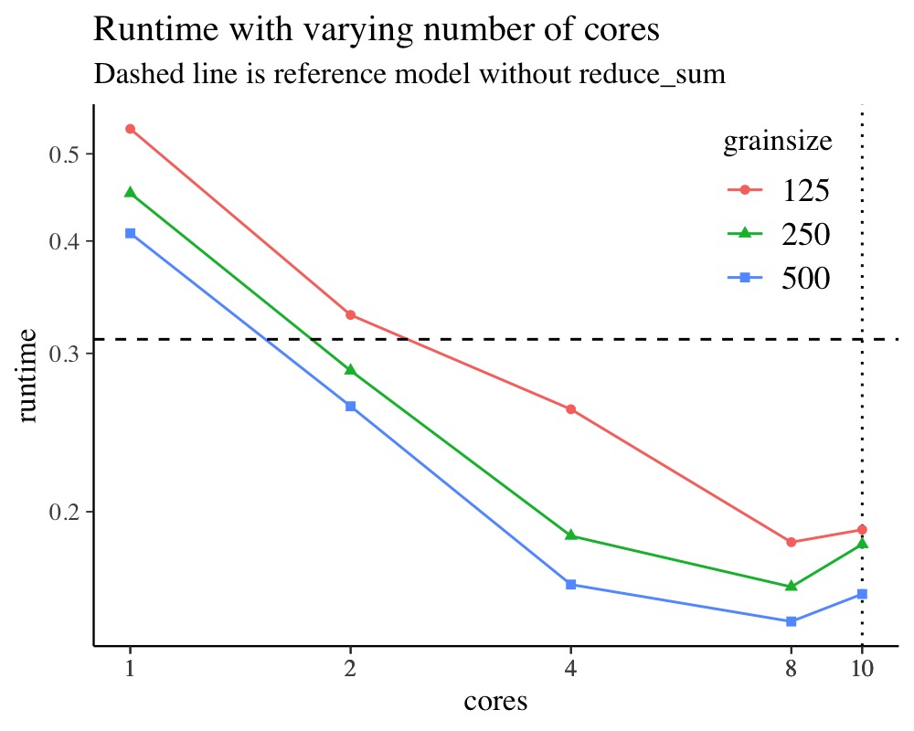
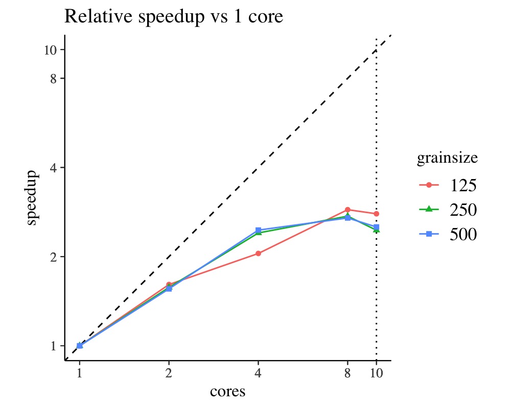
It is important to consider the absolute runtime and the relative speedup vs. running on a single core. The relative speedup can be misleading if the single core runtime is very slow in which case speed gains on more CPUs may look overly good. Considering instead the absolute runtime avoids this problem. After all, we are interested in the shortest walltime we can get rather than any relative speedups.

ggplot(scaling_cores) +
    aes(cores, runtime, shape = grainsize, color = grainsize) +
    geom_vline(xintercept = num_cpu, linetype = 3) +
    geom_line() + geom_point() +
    scale_x_log10(breaks = scaling_cores$cores) +
    scale_y_log10(breaks=seq(0.1, 1.4, by=0.1)) +
    theme(legend.position = c(0.85, 0.8)) +
    geom_hline(data=subset(ref, iter==iter_scaling), aes(yintercept=runtime), linetype=I(2)) +
    ggtitle("Runtime with varying number of cores",
            "Dashed line is reference model without reduce_sum")

ggplot(scaling_cores) +
  aes(cores, speedup, shape = grainsize, color = grainsize) +
  geom_abline(slope = 1, intercept = 0, linetype = 2) +
  geom_vline(xintercept = num_cpu, linetype = 3) +
  geom_line() + geom_point() +
  scale_x_log10(breaks=scaling_cores$cores) +
  scale_y_log10(breaks=scaling_cores$cores) +
  theme(aspect.ratio = 1) +
  coord_fixed(xlim = c(1, num_cpu_logical), ylim = c(1, num_cpu_logical)) +
  ggtitle("Relative speedup vs 1 core")

The vertical dotted line marks the physical number of CPU cores on the machine this was run. The horizontal dashed line in the plot with absolute runtime marks the respective runtime of the model without reduce_sum and the dashed unity line in the plot with the relative speedup marks the theoretical maximal speedup. We can see that there is no further reduction in execution time when increasing the thread count to be greater than the number of physical CPUs. Hence, the use of hyper-threading is not helpful when aiming to maximize the speed of a Stan program. Moreover, the use of threading outperforms the single core runtime only when using more than 4 cores in this example.

For this example, the shown grainsizes matter on some machines but not on others, so your results may look quite different from what is shown here. The overall speedups may not seem impressive in this case, which is attributed in this case to the large number of parameters relative to the number of observations. However, we can still outperform the single core runtime when using many cores. Though the most important advantage of threading is that with an increasing data set size, the user has the option to use a brute-force approach to balance the increase in walltime needed.

kable(scaling_cores, digits = 2)

grainsize	iter	cores	num_leapfrog	runtime	runtime_single	speedup
125	20	1	620	0.53	0.53	1.00
125	20	2	620	0.33	0.53	1.61
125	20	4	620	0.26	0.53	2.05
125	20	8	620	0.18	0.53	2.88
125	20	10	620	0.19	0.53	2.79
250	20	1	620	0.45	0.45	1.00
250	20	2	620	0.29	0.45	1.57
250	20	4	620	0.19	0.45	2.40
250	20	8	620	0.16	0.45	2.74
250	20	10	620	0.18	0.45	2.46
500	20	1	620	0.41	0.41	1.00
500	20	2	620	0.26	0.41	1.56
500	20	4	620	0.17	0.41	2.46
500	20	8	620	0.15	0.41	2.70
500	20	10	620	0.16	0.41	2.52

For a given Stan model one should usually choose the number of chains and the number of threads per chain to be equal to the number of (physical) cores one wishes to use. Only if different chains of the model have relatively different execution times (which they should not have, but it occurs sometimes in practice), then one may consider the use of hyper-threading. Doing so will share the resources evenly across all chains and whenever the fastest chain finishes, the freed resources can be given to the still running chains.

Appendix

Fake data simulation

set.seed(54647)
# number of observations
N <- 1E4
# number of group levels
G <- round(N / 10)
# number of predictors
P <- 3
# regression coefficients
beta <- rnorm(P)

# sampled covariates, group means and fake data
fake <- matrix(rnorm(N * P), ncol = P)
dimnames(fake) <- list(NULL, paste0("x", 1:P))

# fixed effect part and sampled group membership
fake <- transform(
  as.data.frame(fake),
  theta = fake %*% beta,
  g = sample.int(G, N, replace=TRUE)
)

# add random intercept by group
fake  <- merge(fake, data.frame(g = 1:G, eta = rnorm(G)), by = "g")

# linear predictor
fake  <- transform(fake, mu = theta + eta)

# sample Poisson data
fake  <- transform(fake, y = rpois(N, exp(mu)))

# shuffle order of data rows to ensure even distribution of computational effort
fake <- fake[sample.int(N, N),]

# drop not needed row names
rownames(fake) <- NULL

Poisson example model

model_poisson <- brm(
  y ~ 1 + x1 + x2 + (1 | g),
  data = fake,
  family = poisson(),
  iter = 500, # short sampling to speedup example
  chains = 2,
  prior = prior(normal(0,1), class = b) +
    prior(constant(1), class = sd, group = g),
  backend = "cmdstanr",
  threads = threading(4),
  save_pars = save_pars(all = TRUE)
)

Threading benchmark function

# Benchmarks given model with cross-product of tuning parameters CPU
# cores, grainsize and iterations. Models are run with either static
# or non-static scheduler and initial values are set by default to 0 on the
# unconstrained scale. Function returns a data-frame with the
# cross-product of the tuning parameters and as result column the
# respective runtime.
benchmark_threading <- function(model, cores = 1, grainsize = 1, iter = 100,
                                static = FALSE) {

    winfo <- extract_warmup_info(model)
    sims  <- rstan::extract(model$fit)
    init <- list(extract_draw(sims, 1))

    scaling_model <- update(
        model, refresh = 0,
        threads = threading(1, grainsize = grainsize[1], static = static),
        chains = 1, iter = 2, backend = "cmdstanr"
    )

    run_benchmark <- function(cores, size, iter) {
        bench_fit <- update(
            scaling_model, warmup=0, iter = iter,
            chains = 1, seed = 1234, init = init, refresh = 0, save_warmup=TRUE,
            threads = threading(cores, grainsize = size, static = static),
            inv_metric=winfo$inv_metric[[1]],
            step_size=winfo$step_size[[1]],
            adapt_engaged=FALSE
        )
        lf <- sum(subset(nuts_params(bench_fit, inc_warmup=TRUE), Parameter=="n_leapfrog__")$Value)
        elapsed <- sum(colSums(rstan::get_elapsed_time(bench_fit$fit)))

        c(num_leapfrog=lf, runtime=elapsed)
    }

    cases <- expand.grid(cores = cores, grainsize = grainsize, iter = iter)
    res <- with(cases, mapply(run_benchmark, cores, grainsize, iter))
    cbind(cases, as.data.frame(t(res)))
}

benchmark_reference <- function(model, iter=100, init=0) {
    winfo <- extract_warmup_info(model)
    sims  <- rstan::extract(model$fit)
    init <- list(extract_draw(sims, 1))

    ref_model <- update(
        model, refresh = 0, threads = NULL,
        chains = 1, iter = 2, backend = "cmdstanr"
    )

    run_benchmark_ref <- function(iter_bench) {
        bench_fit <- update(
            ref_model, warmup=0, iter = iter_bench,
            chains = 1, seed = 1234, init = init, refresh = 0,
            inv_metric=winfo$inv_metric[[1]],
            step_size=winfo$step_size[[1]],
            adapt_engaged=FALSE
        )

        lf <- sum(subset(nuts_params(bench_fit, inc_warmup=TRUE), Parameter=="n_leapfrog__")$Value)
        elapsed <- sum(colSums(rstan::get_elapsed_time(bench_fit$fit)))

        c(num_leapfrog=lf, runtime=elapsed)
    }

    ref <- sapply(iter, run_benchmark_ref)
    ref <- cbind(as.data.frame(t(ref)), iter=iter)
    ref
}

extract_warmup_info <- function(bfit) {
    adapt  <- lapply(rstan::get_adaptation_info(bfit$fit), strsplit, split="\\n")
    step_size  <- lapply(adapt, function(a) as.numeric(strsplit(a[[1]][[1]], " = ")[[1]][2]))
    inv_metric <- lapply(adapt, function(a) as.numeric(strsplit(sub("^# ", "", a[[1]][[3]]), ", ")[[1]]))
    list(step_size=step_size, inv_metric=inv_metric)
}

extract_draw <- function(sims, draw) {
  lapply(sims, brms:::slice, dim = 1, i = draw, drop = TRUE)
}

Munging of slowdown with chunking data

scaling_chunking <- merge(scaling_chunking, chunking_bench, by = "grainsize")

single_chunk  <- transform(
    subset(scaling_chunking, chunks == 1),
    num_leapfrog_single = num_leapfrog, num_leapfrog = NULL,
    runtime_single = runtime, runtime = NULL,
    grainsize = NULL, chunks=NULL
)

scaling_chunking <- transform(
    merge(scaling_chunking, single_chunk),
    slowdown = runtime/runtime_single,
    iter = factor(iter),
    runtime_single = NULL
)

ref <- transform(ref, iter=factor(iter))

Sebastian Weber & Paul Bürkner

2024-03-19