
Specify a monotonic predictor term in brms. The function does not evaluate its arguments – it exists purely to help set up a model.
Arguments
- x
An integer variable or an ordered factor to be modeled as monotonic.
- id
Optional character string. All monotonic terms with the same
idwithin one formula will be modeled as having the same simplex (shape) parameter vector. If all monotonic terms of the same predictor have the sameid, the resulting predictions will be conditionally monotonic for all values of interacting covariates (Bürkner & Charpentier, 2020).
Details
See Bürkner and Charpentier (2020) for the underlying theory. For
detailed documentation of the formula syntax used for monotonic terms,
see help(brmsformula) as well as vignette("brms_monotonic").
References
Bürkner P. C. & Charpentier E. (2020). Modeling Monotonic Effects of Ordinal Predictors in Regression Models. British Journal of Mathematical and Statistical Psychology. doi:10.1111/bmsp.12195
Examples
# \dontrun{
# generate some data
income_options <- c("below_20", "20_to_40", "40_to_100", "greater_100")
income <- factor(sample(income_options, 100, TRUE),
levels = income_options, ordered = TRUE)
mean_ls <- c(30, 60, 70, 75)
ls <- mean_ls[income] + rnorm(100, sd = 7)
dat <- data.frame(income, ls)
# fit a simple monotonic model
fit1 <- brm(ls ~ mo(income), data = dat)
#> Compiling Stan program...
#> Start sampling
#>
#> SAMPLING FOR MODEL 'anon_model' NOW (CHAIN 1).
#> Chain 1:
#> Chain 1: Gradient evaluation took 2.3e-05 seconds
#> Chain 1: 1000 transitions using 10 leapfrog steps per transition would take 0.23 seconds.
#> Chain 1: Adjust your expectations accordingly!
#> Chain 1:
#> Chain 1:
#> Chain 1: Iteration: 1 / 2000 [ 0%] (Warmup)
#> Chain 1: Iteration: 200 / 2000 [ 10%] (Warmup)
#> Chain 1: Iteration: 400 / 2000 [ 20%] (Warmup)
#> Chain 1: Iteration: 600 / 2000 [ 30%] (Warmup)
#> Chain 1: Iteration: 800 / 2000 [ 40%] (Warmup)
#> Chain 1: Iteration: 1000 / 2000 [ 50%] (Warmup)
#> Chain 1: Iteration: 1001 / 2000 [ 50%] (Sampling)
#> Chain 1: Iteration: 1200 / 2000 [ 60%] (Sampling)
#> Chain 1: Iteration: 1400 / 2000 [ 70%] (Sampling)
#> Chain 1: Iteration: 1600 / 2000 [ 80%] (Sampling)
#> Chain 1: Iteration: 1800 / 2000 [ 90%] (Sampling)
#> Chain 1: Iteration: 2000 / 2000 [100%] (Sampling)
#> Chain 1:
#> Chain 1: Elapsed Time: 0.216 seconds (Warm-up)
#> Chain 1: 0.191 seconds (Sampling)
#> Chain 1: 0.407 seconds (Total)
#> Chain 1:
#>
#> SAMPLING FOR MODEL 'anon_model' NOW (CHAIN 2).
#> Chain 2:
#> Chain 2: Gradient evaluation took 1.9e-05 seconds
#> Chain 2: 1000 transitions using 10 leapfrog steps per transition would take 0.19 seconds.
#> Chain 2: Adjust your expectations accordingly!
#> Chain 2:
#> Chain 2:
#> Chain 2: Iteration: 1 / 2000 [ 0%] (Warmup)
#> Chain 2: Iteration: 200 / 2000 [ 10%] (Warmup)
#> Chain 2: Iteration: 400 / 2000 [ 20%] (Warmup)
#> Chain 2: Iteration: 600 / 2000 [ 30%] (Warmup)
#> Chain 2: Iteration: 800 / 2000 [ 40%] (Warmup)
#> Chain 2: Iteration: 1000 / 2000 [ 50%] (Warmup)
#> Chain 2: Iteration: 1001 / 2000 [ 50%] (Sampling)
#> Chain 2: Iteration: 1200 / 2000 [ 60%] (Sampling)
#> Chain 2: Iteration: 1400 / 2000 [ 70%] (Sampling)
#> Chain 2: Iteration: 1600 / 2000 [ 80%] (Sampling)
#> Chain 2: Iteration: 1800 / 2000 [ 90%] (Sampling)
#> Chain 2: Iteration: 2000 / 2000 [100%] (Sampling)
#> Chain 2:
#> Chain 2: Elapsed Time: 0.229 seconds (Warm-up)
#> Chain 2: 0.224 seconds (Sampling)
#> Chain 2: 0.453 seconds (Total)
#> Chain 2:
#>
#> SAMPLING FOR MODEL 'anon_model' NOW (CHAIN 3).
#> Chain 3:
#> Chain 3: Gradient evaluation took 1.8e-05 seconds
#> Chain 3: 1000 transitions using 10 leapfrog steps per transition would take 0.18 seconds.
#> Chain 3: Adjust your expectations accordingly!
#> Chain 3:
#> Chain 3:
#> Chain 3: Iteration: 1 / 2000 [ 0%] (Warmup)
#> Chain 3: Iteration: 200 / 2000 [ 10%] (Warmup)
#> Chain 3: Iteration: 400 / 2000 [ 20%] (Warmup)
#> Chain 3: Iteration: 600 / 2000 [ 30%] (Warmup)
#> Chain 3: Iteration: 800 / 2000 [ 40%] (Warmup)
#> Chain 3: Iteration: 1000 / 2000 [ 50%] (Warmup)
#> Chain 3: Iteration: 1001 / 2000 [ 50%] (Sampling)
#> Chain 3: Iteration: 1200 / 2000 [ 60%] (Sampling)
#> Chain 3: Iteration: 1400 / 2000 [ 70%] (Sampling)
#> Chain 3: Iteration: 1600 / 2000 [ 80%] (Sampling)
#> Chain 3: Iteration: 1800 / 2000 [ 90%] (Sampling)
#> Chain 3: Iteration: 2000 / 2000 [100%] (Sampling)
#> Chain 3:
#> Chain 3: Elapsed Time: 0.205 seconds (Warm-up)
#> Chain 3: 0.198 seconds (Sampling)
#> Chain 3: 0.403 seconds (Total)
#> Chain 3:
#>
#> SAMPLING FOR MODEL 'anon_model' NOW (CHAIN 4).
#> Chain 4:
#> Chain 4: Gradient evaluation took 1.9e-05 seconds
#> Chain 4: 1000 transitions using 10 leapfrog steps per transition would take 0.19 seconds.
#> Chain 4: Adjust your expectations accordingly!
#> Chain 4:
#> Chain 4:
#> Chain 4: Iteration: 1 / 2000 [ 0%] (Warmup)
#> Chain 4: Iteration: 200 / 2000 [ 10%] (Warmup)
#> Chain 4: Iteration: 400 / 2000 [ 20%] (Warmup)
#> Chain 4: Iteration: 600 / 2000 [ 30%] (Warmup)
#> Chain 4: Iteration: 800 / 2000 [ 40%] (Warmup)
#> Chain 4: Iteration: 1000 / 2000 [ 50%] (Warmup)
#> Chain 4: Iteration: 1001 / 2000 [ 50%] (Sampling)
#> Chain 4: Iteration: 1200 / 2000 [ 60%] (Sampling)
#> Chain 4: Iteration: 1400 / 2000 [ 70%] (Sampling)
#> Chain 4: Iteration: 1600 / 2000 [ 80%] (Sampling)
#> Chain 4: Iteration: 1800 / 2000 [ 90%] (Sampling)
#> Chain 4: Iteration: 2000 / 2000 [100%] (Sampling)
#> Chain 4:
#> Chain 4: Elapsed Time: 0.219 seconds (Warm-up)
#> Chain 4: 0.236 seconds (Sampling)
#> Chain 4: 0.455 seconds (Total)
#> Chain 4:
summary(fit1)
#> Family: gaussian
#> Links: mu = identity
#> Formula: ls ~ mo(income)
#> Data: dat (Number of observations: 100)
#> Draws: 4 chains, each with iter = 2000; warmup = 1000; thin = 1;
#> total post-warmup draws = 4000
#>
#> Regression Coefficients:
#> Estimate Est.Error l-95% CI u-95% CI Rhat Bulk_ESS Tail_ESS
#> Intercept 29.38 1.44 26.55 32.21 1.00 2276 2472
#> moincome 15.12 0.66 13.85 16.42 1.00 1996 2448
#>
#> Monotonic Simplex Parameters:
#> Estimate Est.Error l-95% CI u-95% CI Rhat Bulk_ESS Tail_ESS
#> moincome1[1] 0.64 0.04 0.57 0.71 1.00 3559 2672
#> moincome1[2] 0.28 0.04 0.20 0.37 1.00 2692 2459
#> moincome1[3] 0.08 0.04 0.01 0.15 1.00 2164 1333
#>
#> Further Distributional Parameters:
#> Estimate Est.Error l-95% CI u-95% CI Rhat Bulk_ESS Tail_ESS
#> sigma 7.05 0.53 6.11 8.17 1.00 2771 2405
#>
#> Draws were sampled using sampling(NUTS). For each parameter, Bulk_ESS
#> and Tail_ESS are effective sample size measures, and Rhat is the potential
#> scale reduction factor on split chains (at convergence, Rhat = 1).
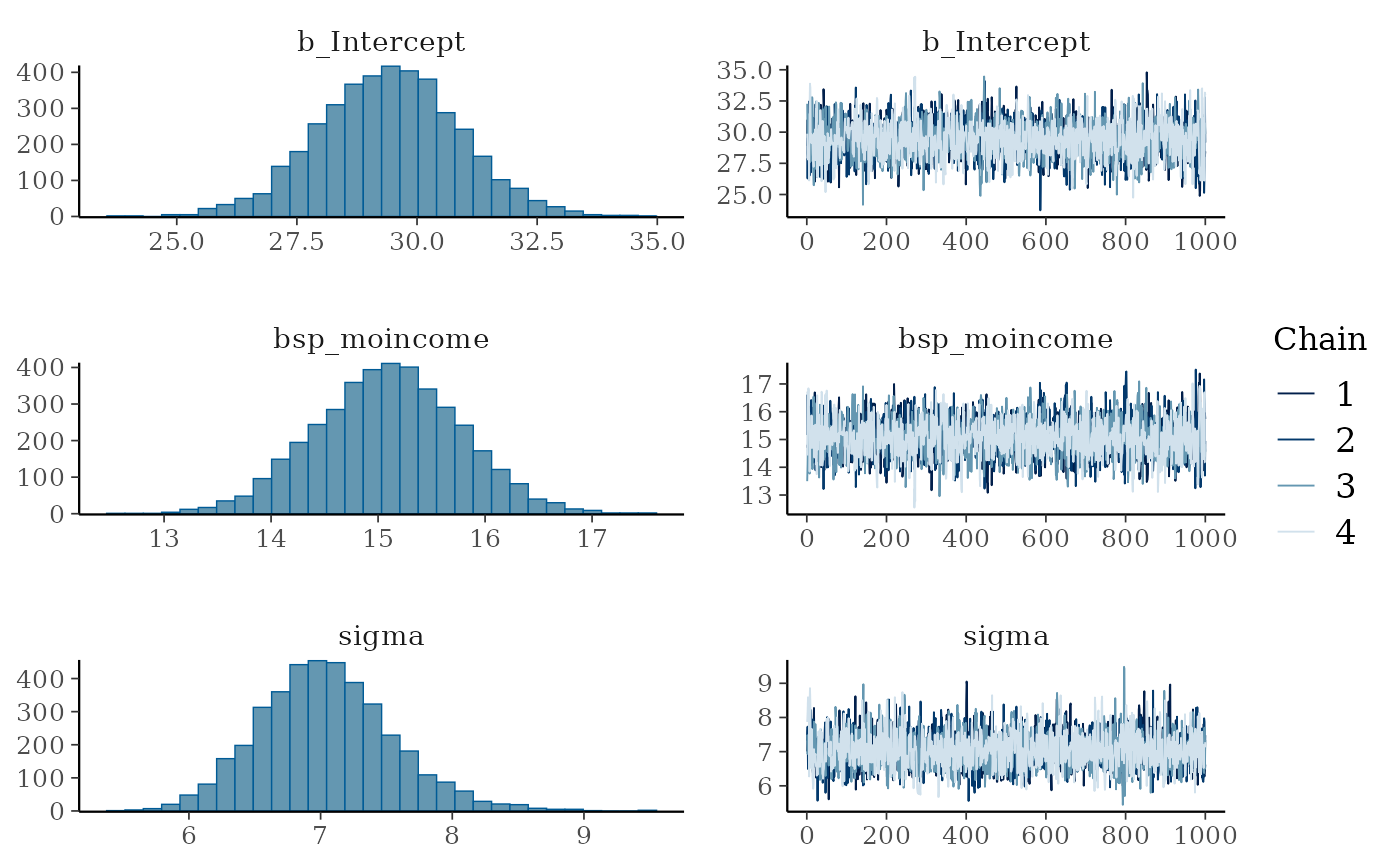
plot(fit1, N = 6)
#> Warning: Argument 'N' is deprecated. Please use argument 'nvariables' instead.
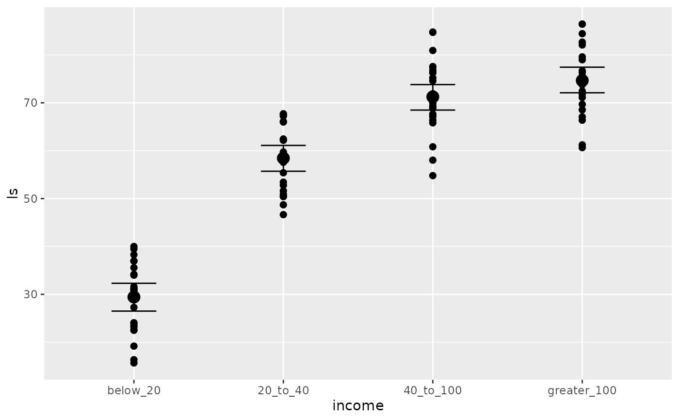
 plot(conditional_effects(fit1), points = TRUE)
 # model interaction with other variables
dat$x <- sample(c("a", "b", "c"), 100, TRUE)
fit2 <- brm(ls ~ mo(income)*x, data = dat)
#> Compiling Stan program...
#> Start sampling
#>
#> SAMPLING FOR MODEL 'anon_model' NOW (CHAIN 1).
#> Chain 1:
#> Chain 1: Gradient evaluation took 4.9e-05 seconds
#> Chain 1: 1000 transitions using 10 leapfrog steps per transition would take 0.49 seconds.
#> Chain 1: Adjust your expectations accordingly!
#> Chain 1:
#> Chain 1:
#> Chain 1: Iteration: 1 / 2000 [ 0%] (Warmup)
#> Chain 1: Iteration: 200 / 2000 [ 10%] (Warmup)
#> Chain 1: Iteration: 400 / 2000 [ 20%] (Warmup)
#> Chain 1: Iteration: 600 / 2000 [ 30%] (Warmup)
#> Chain 1: Iteration: 800 / 2000 [ 40%] (Warmup)
#> Chain 1: Iteration: 1000 / 2000 [ 50%] (Warmup)
#> Chain 1: Iteration: 1001 / 2000 [ 50%] (Sampling)
#> Chain 1: Iteration: 1200 / 2000 [ 60%] (Sampling)
#> Chain 1: Iteration: 1400 / 2000 [ 70%] (Sampling)
#> Chain 1: Iteration: 1600 / 2000 [ 80%] (Sampling)
#> Chain 1: Iteration: 1800 / 2000 [ 90%] (Sampling)
#> Chain 1: Iteration: 2000 / 2000 [100%] (Sampling)
#> Chain 1:
#> Chain 1: Elapsed Time: 1.012 seconds (Warm-up)
#> Chain 1: 0.767 seconds (Sampling)
#> Chain 1: 1.779 seconds (Total)
#> Chain 1:
#>
#> SAMPLING FOR MODEL 'anon_model' NOW (CHAIN 2).
#> Chain 2:
#> Chain 2: Gradient evaluation took 4.4e-05 seconds
#> Chain 2: 1000 transitions using 10 leapfrog steps per transition would take 0.44 seconds.
#> Chain 2: Adjust your expectations accordingly!
#> Chain 2:
#> Chain 2:
#> Chain 2: Iteration: 1 / 2000 [ 0%] (Warmup)
#> Chain 2: Iteration: 200 / 2000 [ 10%] (Warmup)
#> Chain 2: Iteration: 400 / 2000 [ 20%] (Warmup)
#> Chain 2: Iteration: 600 / 2000 [ 30%] (Warmup)
#> Chain 2: Iteration: 800 / 2000 [ 40%] (Warmup)
#> Chain 2: Iteration: 1000 / 2000 [ 50%] (Warmup)
#> Chain 2: Iteration: 1001 / 2000 [ 50%] (Sampling)
#> Chain 2: Iteration: 1200 / 2000 [ 60%] (Sampling)
#> Chain 2: Iteration: 1400 / 2000 [ 70%] (Sampling)
#> Chain 2: Iteration: 1600 / 2000 [ 80%] (Sampling)
#> Chain 2: Iteration: 1800 / 2000 [ 90%] (Sampling)
#> Chain 2: Iteration: 2000 / 2000 [100%] (Sampling)
#> Chain 2:
#> Chain 2: Elapsed Time: 1.013 seconds (Warm-up)
#> Chain 2: 0.712 seconds (Sampling)
#> Chain 2: 1.725 seconds (Total)
#> Chain 2:
#>
#> SAMPLING FOR MODEL 'anon_model' NOW (CHAIN 3).
#> Chain 3:
#> Chain 3: Gradient evaluation took 4.4e-05 seconds
#> Chain 3: 1000 transitions using 10 leapfrog steps per transition would take 0.44 seconds.
#> Chain 3: Adjust your expectations accordingly!
#> Chain 3:
#> Chain 3:
#> Chain 3: Iteration: 1 / 2000 [ 0%] (Warmup)
#> Chain 3: Iteration: 200 / 2000 [ 10%] (Warmup)
#> Chain 3: Iteration: 400 / 2000 [ 20%] (Warmup)
#> Chain 3: Iteration: 600 / 2000 [ 30%] (Warmup)
#> Chain 3: Iteration: 800 / 2000 [ 40%] (Warmup)
#> Chain 3: Iteration: 1000 / 2000 [ 50%] (Warmup)
#> Chain 3: Iteration: 1001 / 2000 [ 50%] (Sampling)
#> Chain 3: Iteration: 1200 / 2000 [ 60%] (Sampling)
#> Chain 3: Iteration: 1400 / 2000 [ 70%] (Sampling)
#> Chain 3: Iteration: 1600 / 2000 [ 80%] (Sampling)
#> Chain 3: Iteration: 1800 / 2000 [ 90%] (Sampling)
#> Chain 3: Iteration: 2000 / 2000 [100%] (Sampling)
#> Chain 3:
#> Chain 3: Elapsed Time: 1.018 seconds (Warm-up)
#> Chain 3: 0.644 seconds (Sampling)
#> Chain 3: 1.662 seconds (Total)
#> Chain 3:
#>
#> SAMPLING FOR MODEL 'anon_model' NOW (CHAIN 4).
#> Chain 4:
#> Chain 4: Gradient evaluation took 7e-05 seconds
#> Chain 4: 1000 transitions using 10 leapfrog steps per transition would take 0.7 seconds.
#> Chain 4: Adjust your expectations accordingly!
#> Chain 4:
#> Chain 4:
#> Chain 4: Iteration: 1 / 2000 [ 0%] (Warmup)
#> Chain 4: Iteration: 200 / 2000 [ 10%] (Warmup)
#> Chain 4: Iteration: 400 / 2000 [ 20%] (Warmup)
#> Chain 4: Iteration: 600 / 2000 [ 30%] (Warmup)
#> Chain 4: Iteration: 800 / 2000 [ 40%] (Warmup)
#> Chain 4: Iteration: 1000 / 2000 [ 50%] (Warmup)
#> Chain 4: Iteration: 1001 / 2000 [ 50%] (Sampling)
#> Chain 4: Iteration: 1200 / 2000 [ 60%] (Sampling)
#> Chain 4: Iteration: 1400 / 2000 [ 70%] (Sampling)
#> Chain 4: Iteration: 1600 / 2000 [ 80%] (Sampling)
#> Chain 4: Iteration: 1800 / 2000 [ 90%] (Sampling)
#> Chain 4: Iteration: 2000 / 2000 [100%] (Sampling)
#> Chain 4:
#> Chain 4: Elapsed Time: 0.953 seconds (Warm-up)
#> Chain 4: 0.62 seconds (Sampling)
#> Chain 4: 1.573 seconds (Total)
#> Chain 4:
summary(fit2)
#> Family: gaussian
#> Links: mu = identity
#> Formula: ls ~ mo(income) * x
#> Data: dat (Number of observations: 100)
#> Draws: 4 chains, each with iter = 2000; warmup = 1000; thin = 1;
#> total post-warmup draws = 4000
#>
#> Regression Coefficients:
#> Estimate Est.Error l-95% CI u-95% CI Rhat Bulk_ESS Tail_ESS
#> Intercept 29.63 1.91 25.95 33.39 1.00 2065 2471
#> xb 1.50 2.82 -4.29 6.97 1.00 1783 2360
#> xc -2.40 2.82 -8.17 2.92 1.00 1895 2569
#> moincome 15.60 0.98 13.71 17.58 1.00 1526 2204
#> moincome:xb -1.27 1.51 -4.22 1.84 1.00 1443 1904
#> moincome:xc -0.40 1.52 -3.34 2.55 1.00 1711 2582
#>
#> Monotonic Simplex Parameters:
#> Estimate Est.Error l-95% CI u-95% CI Rhat Bulk_ESS Tail_ESS
#> moincome1[1] 0.63 0.04 0.55 0.72 1.00 2638 3093
#> moincome1[2] 0.29 0.04 0.20 0.37 1.00 2980 2929
#> moincome1[3] 0.08 0.04 0.01 0.16 1.00 1961 1379
#> moincome:xb1[1] 0.28 0.22 0.01 0.79 1.00 2625 2251
#> moincome:xb1[2] 0.32 0.23 0.01 0.82 1.00 4237 2560
#> moincome:xb1[3] 0.40 0.25 0.02 0.87 1.00 2924 2222
#> moincome:xc1[1] 0.34 0.23 0.01 0.83 1.00 3014 1792
#> moincome:xc1[2] 0.32 0.23 0.01 0.82 1.00 3896 2067
#> moincome:xc1[3] 0.35 0.23 0.01 0.85 1.00 3549 2068
#>
#> Further Distributional Parameters:
#> Estimate Est.Error l-95% CI u-95% CI Rhat Bulk_ESS Tail_ESS
#> sigma 7.03 0.52 6.11 8.15 1.00 4209 3037
#>
#> Draws were sampled using sampling(NUTS). For each parameter, Bulk_ESS
#> and Tail_ESS are effective sample size measures, and Rhat is the potential
#> scale reduction factor on split chains (at convergence, Rhat = 1).
plot(conditional_effects(fit2), points = TRUE)
# model interaction with other variables
dat$x <- sample(c("a", "b", "c"), 100, TRUE)
fit2 <- brm(ls ~ mo(income)*x, data = dat)
#> Compiling Stan program...
#> Start sampling
#>
#> SAMPLING FOR MODEL 'anon_model' NOW (CHAIN 1).
#> Chain 1:
#> Chain 1: Gradient evaluation took 4.9e-05 seconds
#> Chain 1: 1000 transitions using 10 leapfrog steps per transition would take 0.49 seconds.
#> Chain 1: Adjust your expectations accordingly!
#> Chain 1:
#> Chain 1:
#> Chain 1: Iteration: 1 / 2000 [ 0%] (Warmup)
#> Chain 1: Iteration: 200 / 2000 [ 10%] (Warmup)
#> Chain 1: Iteration: 400 / 2000 [ 20%] (Warmup)
#> Chain 1: Iteration: 600 / 2000 [ 30%] (Warmup)
#> Chain 1: Iteration: 800 / 2000 [ 40%] (Warmup)
#> Chain 1: Iteration: 1000 / 2000 [ 50%] (Warmup)
#> Chain 1: Iteration: 1001 / 2000 [ 50%] (Sampling)
#> Chain 1: Iteration: 1200 / 2000 [ 60%] (Sampling)
#> Chain 1: Iteration: 1400 / 2000 [ 70%] (Sampling)
#> Chain 1: Iteration: 1600 / 2000 [ 80%] (Sampling)
#> Chain 1: Iteration: 1800 / 2000 [ 90%] (Sampling)
#> Chain 1: Iteration: 2000 / 2000 [100%] (Sampling)
#> Chain 1:
#> Chain 1: Elapsed Time: 1.012 seconds (Warm-up)
#> Chain 1: 0.767 seconds (Sampling)
#> Chain 1: 1.779 seconds (Total)
#> Chain 1:
#>
#> SAMPLING FOR MODEL 'anon_model' NOW (CHAIN 2).
#> Chain 2:
#> Chain 2: Gradient evaluation took 4.4e-05 seconds
#> Chain 2: 1000 transitions using 10 leapfrog steps per transition would take 0.44 seconds.
#> Chain 2: Adjust your expectations accordingly!
#> Chain 2:
#> Chain 2:
#> Chain 2: Iteration: 1 / 2000 [ 0%] (Warmup)
#> Chain 2: Iteration: 200 / 2000 [ 10%] (Warmup)
#> Chain 2: Iteration: 400 / 2000 [ 20%] (Warmup)
#> Chain 2: Iteration: 600 / 2000 [ 30%] (Warmup)
#> Chain 2: Iteration: 800 / 2000 [ 40%] (Warmup)
#> Chain 2: Iteration: 1000 / 2000 [ 50%] (Warmup)
#> Chain 2: Iteration: 1001 / 2000 [ 50%] (Sampling)
#> Chain 2: Iteration: 1200 / 2000 [ 60%] (Sampling)
#> Chain 2: Iteration: 1400 / 2000 [ 70%] (Sampling)
#> Chain 2: Iteration: 1600 / 2000 [ 80%] (Sampling)
#> Chain 2: Iteration: 1800 / 2000 [ 90%] (Sampling)
#> Chain 2: Iteration: 2000 / 2000 [100%] (Sampling)
#> Chain 2:
#> Chain 2: Elapsed Time: 1.013 seconds (Warm-up)
#> Chain 2: 0.712 seconds (Sampling)
#> Chain 2: 1.725 seconds (Total)
#> Chain 2:
#>
#> SAMPLING FOR MODEL 'anon_model' NOW (CHAIN 3).
#> Chain 3:
#> Chain 3: Gradient evaluation took 4.4e-05 seconds
#> Chain 3: 1000 transitions using 10 leapfrog steps per transition would take 0.44 seconds.
#> Chain 3: Adjust your expectations accordingly!
#> Chain 3:
#> Chain 3:
#> Chain 3: Iteration: 1 / 2000 [ 0%] (Warmup)
#> Chain 3: Iteration: 200 / 2000 [ 10%] (Warmup)
#> Chain 3: Iteration: 400 / 2000 [ 20%] (Warmup)
#> Chain 3: Iteration: 600 / 2000 [ 30%] (Warmup)
#> Chain 3: Iteration: 800 / 2000 [ 40%] (Warmup)
#> Chain 3: Iteration: 1000 / 2000 [ 50%] (Warmup)
#> Chain 3: Iteration: 1001 / 2000 [ 50%] (Sampling)
#> Chain 3: Iteration: 1200 / 2000 [ 60%] (Sampling)
#> Chain 3: Iteration: 1400 / 2000 [ 70%] (Sampling)
#> Chain 3: Iteration: 1600 / 2000 [ 80%] (Sampling)
#> Chain 3: Iteration: 1800 / 2000 [ 90%] (Sampling)
#> Chain 3: Iteration: 2000 / 2000 [100%] (Sampling)
#> Chain 3:
#> Chain 3: Elapsed Time: 1.018 seconds (Warm-up)
#> Chain 3: 0.644 seconds (Sampling)
#> Chain 3: 1.662 seconds (Total)
#> Chain 3:
#>
#> SAMPLING FOR MODEL 'anon_model' NOW (CHAIN 4).
#> Chain 4:
#> Chain 4: Gradient evaluation took 7e-05 seconds
#> Chain 4: 1000 transitions using 10 leapfrog steps per transition would take 0.7 seconds.
#> Chain 4: Adjust your expectations accordingly!
#> Chain 4:
#> Chain 4:
#> Chain 4: Iteration: 1 / 2000 [ 0%] (Warmup)
#> Chain 4: Iteration: 200 / 2000 [ 10%] (Warmup)
#> Chain 4: Iteration: 400 / 2000 [ 20%] (Warmup)
#> Chain 4: Iteration: 600 / 2000 [ 30%] (Warmup)
#> Chain 4: Iteration: 800 / 2000 [ 40%] (Warmup)
#> Chain 4: Iteration: 1000 / 2000 [ 50%] (Warmup)
#> Chain 4: Iteration: 1001 / 2000 [ 50%] (Sampling)
#> Chain 4: Iteration: 1200 / 2000 [ 60%] (Sampling)
#> Chain 4: Iteration: 1400 / 2000 [ 70%] (Sampling)
#> Chain 4: Iteration: 1600 / 2000 [ 80%] (Sampling)
#> Chain 4: Iteration: 1800 / 2000 [ 90%] (Sampling)
#> Chain 4: Iteration: 2000 / 2000 [100%] (Sampling)
#> Chain 4:
#> Chain 4: Elapsed Time: 0.953 seconds (Warm-up)
#> Chain 4: 0.62 seconds (Sampling)
#> Chain 4: 1.573 seconds (Total)
#> Chain 4:
summary(fit2)
#> Family: gaussian
#> Links: mu = identity
#> Formula: ls ~ mo(income) * x
#> Data: dat (Number of observations: 100)
#> Draws: 4 chains, each with iter = 2000; warmup = 1000; thin = 1;
#> total post-warmup draws = 4000
#>
#> Regression Coefficients:
#> Estimate Est.Error l-95% CI u-95% CI Rhat Bulk_ESS Tail_ESS
#> Intercept 29.63 1.91 25.95 33.39 1.00 2065 2471
#> xb 1.50 2.82 -4.29 6.97 1.00 1783 2360
#> xc -2.40 2.82 -8.17 2.92 1.00 1895 2569
#> moincome 15.60 0.98 13.71 17.58 1.00 1526 2204
#> moincome:xb -1.27 1.51 -4.22 1.84 1.00 1443 1904
#> moincome:xc -0.40 1.52 -3.34 2.55 1.00 1711 2582
#>
#> Monotonic Simplex Parameters:
#> Estimate Est.Error l-95% CI u-95% CI Rhat Bulk_ESS Tail_ESS
#> moincome1[1] 0.63 0.04 0.55 0.72 1.00 2638 3093
#> moincome1[2] 0.29 0.04 0.20 0.37 1.00 2980 2929
#> moincome1[3] 0.08 0.04 0.01 0.16 1.00 1961 1379
#> moincome:xb1[1] 0.28 0.22 0.01 0.79 1.00 2625 2251
#> moincome:xb1[2] 0.32 0.23 0.01 0.82 1.00 4237 2560
#> moincome:xb1[3] 0.40 0.25 0.02 0.87 1.00 2924 2222
#> moincome:xc1[1] 0.34 0.23 0.01 0.83 1.00 3014 1792
#> moincome:xc1[2] 0.32 0.23 0.01 0.82 1.00 3896 2067
#> moincome:xc1[3] 0.35 0.23 0.01 0.85 1.00 3549 2068
#>
#> Further Distributional Parameters:
#> Estimate Est.Error l-95% CI u-95% CI Rhat Bulk_ESS Tail_ESS
#> sigma 7.03 0.52 6.11 8.15 1.00 4209 3037
#>
#> Draws were sampled using sampling(NUTS). For each parameter, Bulk_ESS
#> and Tail_ESS are effective sample size measures, and Rhat is the potential
#> scale reduction factor on split chains (at convergence, Rhat = 1).
plot(conditional_effects(fit2), points = TRUE)


 # ensure conditional monotonicity
fit3 <- brm(ls ~ mo(income, id = "i")*x, data = dat)
#> Compiling Stan program...
#> Start sampling
#>
#> SAMPLING FOR MODEL 'anon_model' NOW (CHAIN 1).
#> Chain 1:
#> Chain 1: Gradient evaluation took 6.9e-05 seconds
#> Chain 1: 1000 transitions using 10 leapfrog steps per transition would take 0.69 seconds.
#> Chain 1: Adjust your expectations accordingly!
#> Chain 1:
#> Chain 1:
#> Chain 1: Iteration: 1 / 2000 [ 0%] (Warmup)
#> Chain 1: Iteration: 200 / 2000 [ 10%] (Warmup)
#> Chain 1: Iteration: 400 / 2000 [ 20%] (Warmup)
#> Chain 1: Iteration: 600 / 2000 [ 30%] (Warmup)
#> Chain 1: Iteration: 800 / 2000 [ 40%] (Warmup)
#> Chain 1: Iteration: 1000 / 2000 [ 50%] (Warmup)
#> Chain 1: Iteration: 1001 / 2000 [ 50%] (Sampling)
#> Chain 1: Iteration: 1200 / 2000 [ 60%] (Sampling)
#> Chain 1: Iteration: 1400 / 2000 [ 70%] (Sampling)
#> Chain 1: Iteration: 1600 / 2000 [ 80%] (Sampling)
#> Chain 1: Iteration: 1800 / 2000 [ 90%] (Sampling)
#> Chain 1: Iteration: 2000 / 2000 [100%] (Sampling)
#> Chain 1:
#> Chain 1: Elapsed Time: 0.981 seconds (Warm-up)
#> Chain 1: 0.859 seconds (Sampling)
#> Chain 1: 1.84 seconds (Total)
#> Chain 1:
#>
#> SAMPLING FOR MODEL 'anon_model' NOW (CHAIN 2).
#> Chain 2:
#> Chain 2: Gradient evaluation took 4.3e-05 seconds
#> Chain 2: 1000 transitions using 10 leapfrog steps per transition would take 0.43 seconds.
#> Chain 2: Adjust your expectations accordingly!
#> Chain 2:
#> Chain 2:
#> Chain 2: Iteration: 1 / 2000 [ 0%] (Warmup)
#> Chain 2: Iteration: 200 / 2000 [ 10%] (Warmup)
#> Chain 2: Iteration: 400 / 2000 [ 20%] (Warmup)
#> Chain 2: Iteration: 600 / 2000 [ 30%] (Warmup)
#> Chain 2: Iteration: 800 / 2000 [ 40%] (Warmup)
#> Chain 2: Iteration: 1000 / 2000 [ 50%] (Warmup)
#> Chain 2: Iteration: 1001 / 2000 [ 50%] (Sampling)
#> Chain 2: Iteration: 1200 / 2000 [ 60%] (Sampling)
#> Chain 2: Iteration: 1400 / 2000 [ 70%] (Sampling)
#> Chain 2: Iteration: 1600 / 2000 [ 80%] (Sampling)
#> Chain 2: Iteration: 1800 / 2000 [ 90%] (Sampling)
#> Chain 2: Iteration: 2000 / 2000 [100%] (Sampling)
#> Chain 2:
#> Chain 2: Elapsed Time: 0.966 seconds (Warm-up)
#> Chain 2: 0.784 seconds (Sampling)
#> Chain 2: 1.75 seconds (Total)
#> Chain 2:
#>
#> SAMPLING FOR MODEL 'anon_model' NOW (CHAIN 3).
#> Chain 3:
#> Chain 3: Gradient evaluation took 4.2e-05 seconds
#> Chain 3: 1000 transitions using 10 leapfrog steps per transition would take 0.42 seconds.
#> Chain 3: Adjust your expectations accordingly!
#> Chain 3:
#> Chain 3:
#> Chain 3: Iteration: 1 / 2000 [ 0%] (Warmup)
#> Chain 3: Iteration: 200 / 2000 [ 10%] (Warmup)
#> Chain 3: Iteration: 400 / 2000 [ 20%] (Warmup)
#> Chain 3: Iteration: 600 / 2000 [ 30%] (Warmup)
#> Chain 3: Iteration: 800 / 2000 [ 40%] (Warmup)
#> Chain 3: Iteration: 1000 / 2000 [ 50%] (Warmup)
#> Chain 3: Iteration: 1001 / 2000 [ 50%] (Sampling)
#> Chain 3: Iteration: 1200 / 2000 [ 60%] (Sampling)
#> Chain 3: Iteration: 1400 / 2000 [ 70%] (Sampling)
#> Chain 3: Iteration: 1600 / 2000 [ 80%] (Sampling)
#> Chain 3: Iteration: 1800 / 2000 [ 90%] (Sampling)
#> Chain 3: Iteration: 2000 / 2000 [100%] (Sampling)
#> Chain 3:
#> Chain 3: Elapsed Time: 1.03 seconds (Warm-up)
#> Chain 3: 0.833 seconds (Sampling)
#> Chain 3: 1.863 seconds (Total)
#> Chain 3:
#>
#> SAMPLING FOR MODEL 'anon_model' NOW (CHAIN 4).
#> Chain 4:
#> Chain 4: Gradient evaluation took 4.2e-05 seconds
#> Chain 4: 1000 transitions using 10 leapfrog steps per transition would take 0.42 seconds.
#> Chain 4: Adjust your expectations accordingly!
#> Chain 4:
#> Chain 4:
#> Chain 4: Iteration: 1 / 2000 [ 0%] (Warmup)
#> Chain 4: Iteration: 200 / 2000 [ 10%] (Warmup)
#> Chain 4: Iteration: 400 / 2000 [ 20%] (Warmup)
#> Chain 4: Iteration: 600 / 2000 [ 30%] (Warmup)
#> Chain 4: Iteration: 800 / 2000 [ 40%] (Warmup)
#> Chain 4: Iteration: 1000 / 2000 [ 50%] (Warmup)
#> Chain 4: Iteration: 1001 / 2000 [ 50%] (Sampling)
#> Chain 4: Iteration: 1200 / 2000 [ 60%] (Sampling)
#> Chain 4: Iteration: 1400 / 2000 [ 70%] (Sampling)
#> Chain 4: Iteration: 1600 / 2000 [ 80%] (Sampling)
#> Chain 4: Iteration: 1800 / 2000 [ 90%] (Sampling)
#> Chain 4: Iteration: 2000 / 2000 [100%] (Sampling)
#> Chain 4:
#> Chain 4: Elapsed Time: 0.946 seconds (Warm-up)
#> Chain 4: 0.763 seconds (Sampling)
#> Chain 4: 1.709 seconds (Total)
#> Chain 4:
summary(fit3)
#> Family: gaussian
#> Links: mu = identity
#> Formula: ls ~ mo(income, id = "i") * x
#> Data: dat (Number of observations: 100)
#> Draws: 4 chains, each with iter = 2000; warmup = 1000; thin = 1;
#> total post-warmup draws = 4000
#>
#> Regression Coefficients:
#> Estimate Est.Error l-95% CI u-95% CI Rhat Bulk_ESS Tail_ESS
#> Intercept 30.09 2.10 25.92 34.26 1.00 2321 2475
#> xb 0.20 3.51 -6.99 6.95 1.00 2212 2178
#> xc -2.96 3.49 -9.85 3.84 1.00 1787 2417
#> moincomeidEQi 15.18 1.01 13.17 17.19 1.00 2003 2426
#> moincomeidEQi:xb -0.19 1.53 -3.18 2.94 1.00 2106 2075
#> moincomeidEQi:xc 0.02 1.53 -2.97 2.92 1.00 1728 2287
#>
#> Monotonic Simplex Parameters:
#> Estimate Est.Error l-95% CI u-95% CI Rhat Bulk_ESS
#> moincomeidEQi1[1] 0.65 0.04 0.57 0.72 1.00 4060
#> moincomeidEQi1[2] 0.28 0.04 0.20 0.37 1.00 2990
#> moincomeidEQi1[3] 0.07 0.04 0.01 0.15 1.00 2912
#> moincomeidEQi:xb1[1] 0.65 0.04 0.57 0.72 1.00 4060
#> moincomeidEQi:xb1[2] 0.28 0.04 0.20 0.37 1.00 2990
#> moincomeidEQi:xb1[3] 0.07 0.04 0.01 0.15 1.00 2912
#> moincomeidEQi:xc1[1] 0.65 0.04 0.57 0.72 1.00 4060
#> moincomeidEQi:xc1[2] 0.28 0.04 0.20 0.37 1.00 2990
#> moincomeidEQi:xc1[3] 0.07 0.04 0.01 0.15 1.00 2912
#> Tail_ESS
#> moincomeidEQi1[1] 2878
#> moincomeidEQi1[2] 2418
#> moincomeidEQi1[3] 1699
#> moincomeidEQi:xb1[1] 2878
#> moincomeidEQi:xb1[2] 2418
#> moincomeidEQi:xb1[3] 1699
#> moincomeidEQi:xc1[1] 2878
#> moincomeidEQi:xc1[2] 2418
#> moincomeidEQi:xc1[3] 1699
#>
#> Further Distributional Parameters:
#> Estimate Est.Error l-95% CI u-95% CI Rhat Bulk_ESS Tail_ESS
#> sigma 7.07 0.52 6.14 8.17 1.00 3205 2871
#>
#> Draws were sampled using sampling(NUTS). For each parameter, Bulk_ESS
#> and Tail_ESS are effective sample size measures, and Rhat is the potential
#> scale reduction factor on split chains (at convergence, Rhat = 1).
plot(conditional_effects(fit3), points = TRUE)
# ensure conditional monotonicity
fit3 <- brm(ls ~ mo(income, id = "i")*x, data = dat)
#> Compiling Stan program...
#> Start sampling
#>
#> SAMPLING FOR MODEL 'anon_model' NOW (CHAIN 1).
#> Chain 1:
#> Chain 1: Gradient evaluation took 6.9e-05 seconds
#> Chain 1: 1000 transitions using 10 leapfrog steps per transition would take 0.69 seconds.
#> Chain 1: Adjust your expectations accordingly!
#> Chain 1:
#> Chain 1:
#> Chain 1: Iteration: 1 / 2000 [ 0%] (Warmup)
#> Chain 1: Iteration: 200 / 2000 [ 10%] (Warmup)
#> Chain 1: Iteration: 400 / 2000 [ 20%] (Warmup)
#> Chain 1: Iteration: 600 / 2000 [ 30%] (Warmup)
#> Chain 1: Iteration: 800 / 2000 [ 40%] (Warmup)
#> Chain 1: Iteration: 1000 / 2000 [ 50%] (Warmup)
#> Chain 1: Iteration: 1001 / 2000 [ 50%] (Sampling)
#> Chain 1: Iteration: 1200 / 2000 [ 60%] (Sampling)
#> Chain 1: Iteration: 1400 / 2000 [ 70%] (Sampling)
#> Chain 1: Iteration: 1600 / 2000 [ 80%] (Sampling)
#> Chain 1: Iteration: 1800 / 2000 [ 90%] (Sampling)
#> Chain 1: Iteration: 2000 / 2000 [100%] (Sampling)
#> Chain 1:
#> Chain 1: Elapsed Time: 0.981 seconds (Warm-up)
#> Chain 1: 0.859 seconds (Sampling)
#> Chain 1: 1.84 seconds (Total)
#> Chain 1:
#>
#> SAMPLING FOR MODEL 'anon_model' NOW (CHAIN 2).
#> Chain 2:
#> Chain 2: Gradient evaluation took 4.3e-05 seconds
#> Chain 2: 1000 transitions using 10 leapfrog steps per transition would take 0.43 seconds.
#> Chain 2: Adjust your expectations accordingly!
#> Chain 2:
#> Chain 2:
#> Chain 2: Iteration: 1 / 2000 [ 0%] (Warmup)
#> Chain 2: Iteration: 200 / 2000 [ 10%] (Warmup)
#> Chain 2: Iteration: 400 / 2000 [ 20%] (Warmup)
#> Chain 2: Iteration: 600 / 2000 [ 30%] (Warmup)
#> Chain 2: Iteration: 800 / 2000 [ 40%] (Warmup)
#> Chain 2: Iteration: 1000 / 2000 [ 50%] (Warmup)
#> Chain 2: Iteration: 1001 / 2000 [ 50%] (Sampling)
#> Chain 2: Iteration: 1200 / 2000 [ 60%] (Sampling)
#> Chain 2: Iteration: 1400 / 2000 [ 70%] (Sampling)
#> Chain 2: Iteration: 1600 / 2000 [ 80%] (Sampling)
#> Chain 2: Iteration: 1800 / 2000 [ 90%] (Sampling)
#> Chain 2: Iteration: 2000 / 2000 [100%] (Sampling)
#> Chain 2:
#> Chain 2: Elapsed Time: 0.966 seconds (Warm-up)
#> Chain 2: 0.784 seconds (Sampling)
#> Chain 2: 1.75 seconds (Total)
#> Chain 2:
#>
#> SAMPLING FOR MODEL 'anon_model' NOW (CHAIN 3).
#> Chain 3:
#> Chain 3: Gradient evaluation took 4.2e-05 seconds
#> Chain 3: 1000 transitions using 10 leapfrog steps per transition would take 0.42 seconds.
#> Chain 3: Adjust your expectations accordingly!
#> Chain 3:
#> Chain 3:
#> Chain 3: Iteration: 1 / 2000 [ 0%] (Warmup)
#> Chain 3: Iteration: 200 / 2000 [ 10%] (Warmup)
#> Chain 3: Iteration: 400 / 2000 [ 20%] (Warmup)
#> Chain 3: Iteration: 600 / 2000 [ 30%] (Warmup)
#> Chain 3: Iteration: 800 / 2000 [ 40%] (Warmup)
#> Chain 3: Iteration: 1000 / 2000 [ 50%] (Warmup)
#> Chain 3: Iteration: 1001 / 2000 [ 50%] (Sampling)
#> Chain 3: Iteration: 1200 / 2000 [ 60%] (Sampling)
#> Chain 3: Iteration: 1400 / 2000 [ 70%] (Sampling)
#> Chain 3: Iteration: 1600 / 2000 [ 80%] (Sampling)
#> Chain 3: Iteration: 1800 / 2000 [ 90%] (Sampling)
#> Chain 3: Iteration: 2000 / 2000 [100%] (Sampling)
#> Chain 3:
#> Chain 3: Elapsed Time: 1.03 seconds (Warm-up)
#> Chain 3: 0.833 seconds (Sampling)
#> Chain 3: 1.863 seconds (Total)
#> Chain 3:
#>
#> SAMPLING FOR MODEL 'anon_model' NOW (CHAIN 4).
#> Chain 4:
#> Chain 4: Gradient evaluation took 4.2e-05 seconds
#> Chain 4: 1000 transitions using 10 leapfrog steps per transition would take 0.42 seconds.
#> Chain 4: Adjust your expectations accordingly!
#> Chain 4:
#> Chain 4:
#> Chain 4: Iteration: 1 / 2000 [ 0%] (Warmup)
#> Chain 4: Iteration: 200 / 2000 [ 10%] (Warmup)
#> Chain 4: Iteration: 400 / 2000 [ 20%] (Warmup)
#> Chain 4: Iteration: 600 / 2000 [ 30%] (Warmup)
#> Chain 4: Iteration: 800 / 2000 [ 40%] (Warmup)
#> Chain 4: Iteration: 1000 / 2000 [ 50%] (Warmup)
#> Chain 4: Iteration: 1001 / 2000 [ 50%] (Sampling)
#> Chain 4: Iteration: 1200 / 2000 [ 60%] (Sampling)
#> Chain 4: Iteration: 1400 / 2000 [ 70%] (Sampling)
#> Chain 4: Iteration: 1600 / 2000 [ 80%] (Sampling)
#> Chain 4: Iteration: 1800 / 2000 [ 90%] (Sampling)
#> Chain 4: Iteration: 2000 / 2000 [100%] (Sampling)
#> Chain 4:
#> Chain 4: Elapsed Time: 0.946 seconds (Warm-up)
#> Chain 4: 0.763 seconds (Sampling)
#> Chain 4: 1.709 seconds (Total)
#> Chain 4:
summary(fit3)
#> Family: gaussian
#> Links: mu = identity
#> Formula: ls ~ mo(income, id = "i") * x
#> Data: dat (Number of observations: 100)
#> Draws: 4 chains, each with iter = 2000; warmup = 1000; thin = 1;
#> total post-warmup draws = 4000
#>
#> Regression Coefficients:
#> Estimate Est.Error l-95% CI u-95% CI Rhat Bulk_ESS Tail_ESS
#> Intercept 30.09 2.10 25.92 34.26 1.00 2321 2475
#> xb 0.20 3.51 -6.99 6.95 1.00 2212 2178
#> xc -2.96 3.49 -9.85 3.84 1.00 1787 2417
#> moincomeidEQi 15.18 1.01 13.17 17.19 1.00 2003 2426
#> moincomeidEQi:xb -0.19 1.53 -3.18 2.94 1.00 2106 2075
#> moincomeidEQi:xc 0.02 1.53 -2.97 2.92 1.00 1728 2287
#>
#> Monotonic Simplex Parameters:
#> Estimate Est.Error l-95% CI u-95% CI Rhat Bulk_ESS
#> moincomeidEQi1[1] 0.65 0.04 0.57 0.72 1.00 4060
#> moincomeidEQi1[2] 0.28 0.04 0.20 0.37 1.00 2990
#> moincomeidEQi1[3] 0.07 0.04 0.01 0.15 1.00 2912
#> moincomeidEQi:xb1[1] 0.65 0.04 0.57 0.72 1.00 4060
#> moincomeidEQi:xb1[2] 0.28 0.04 0.20 0.37 1.00 2990
#> moincomeidEQi:xb1[3] 0.07 0.04 0.01 0.15 1.00 2912
#> moincomeidEQi:xc1[1] 0.65 0.04 0.57 0.72 1.00 4060
#> moincomeidEQi:xc1[2] 0.28 0.04 0.20 0.37 1.00 2990
#> moincomeidEQi:xc1[3] 0.07 0.04 0.01 0.15 1.00 2912
#> Tail_ESS
#> moincomeidEQi1[1] 2878
#> moincomeidEQi1[2] 2418
#> moincomeidEQi1[3] 1699
#> moincomeidEQi:xb1[1] 2878
#> moincomeidEQi:xb1[2] 2418
#> moincomeidEQi:xb1[3] 1699
#> moincomeidEQi:xc1[1] 2878
#> moincomeidEQi:xc1[2] 2418
#> moincomeidEQi:xc1[3] 1699
#>
#> Further Distributional Parameters:
#> Estimate Est.Error l-95% CI u-95% CI Rhat Bulk_ESS Tail_ESS
#> sigma 7.07 0.52 6.14 8.17 1.00 3205 2871
#>
#> Draws were sampled using sampling(NUTS). For each parameter, Bulk_ESS
#> and Tail_ESS are effective sample size measures, and Rhat is the potential
#> scale reduction factor on split chains (at convergence, Rhat = 1).
plot(conditional_effects(fit3), points = TRUE)


 # }
# }