
Estimating Multivariate Models with brms
Paul Bürkner
2026-09-10
Source:vignettes/brms_multivariate.Rmd
brms_multivariate.RmdIntroduction
In the present vignette, we want to discuss how to specify
multivariate multilevel models using brms. We call a
model multivariate if it contains multiple response variables,
each being predicted by its own set of predictors. Consider an example
from biology. Hadfield, Nutall, Osorio, and Owens (2007) analyzed data
of the Eurasian blue tit (https://en.wikipedia.org/wiki/Eurasian_blue_tit). They
predicted the tarsus length as well as the
back color of chicks. Half of the brood were put into
another fosternest, while the other half stayed in the
fosternest of their own dam. This allows to separate
genetic from environmental factors. Additionally, we have information
about the hatchdate and sex of the chicks (the
latter being known for 94% of the animals).
       tarsus       back  animal     dam fosternest  hatchdate  sex
1 -1.89229718  1.1464212 R187142 R187557      F2102 -0.6874021  Fem
2  1.13610981 -0.7596521 R187154 R187559      F1902 -0.6874021 Male
3  0.98468946  0.1449373 R187341 R187568       A602 -0.4279814 Male
4  0.37900806  0.2555847 R046169 R187518      A1302 -1.4656641 Male
5 -0.07525299 -0.3006992 R046161 R187528      A2602 -1.4656641  Fem
6 -1.13519543  1.5577219 R187409 R187945      C2302  0.3502805  Fem
Basic Multivariate Models
We begin with a relatively simple multivariate normal model.
bform1 <-
  bf(mvbind(tarsus, back) ~ sex + hatchdate + (1|p|fosternest) + (1|q|dam)) +
  set_rescor(TRUE)

fit1 <- brm(bform1, data = BTdata, chains = 2, cores = 2)
As can be seen in the model code, we have used mvbind
notation to tell brms that both tarsus and
back are separate response variables. The term
(1|p|fosternest) indicates a varying intercept over
fosternest. By writing |p| in between we
indicate that all varying effects of fosternest should be
modeled as correlated. This makes sense since we actually have two model
parts, one for tarsus and one for back. The
indicator p is arbitrary and can be replaced by other
symbols that comes into your mind (for details about the multilevel
syntax of brms, see help("brmsformula")
and vignette("brms_multilevel")). Similarly, the term
(1|q|dam) indicates correlated varying effects of the
genetic mother of the chicks. Alternatively, we could have also modeled
the genetic similarities through pedigrees and corresponding relatedness
matrices, but this is not the focus of this vignette (please see
vignette("brms_phylogenetics")). The model results are
readily summarized via
fit1 <- add_criterion(fit1, "loo")
summary(fit1)
Family: MV(gaussian, gaussian)
Links: mu = identity
mu = identity
Formula: tarsus ~ sex + hatchdate + (1 | p | fosternest) + (1 | q | dam)
back ~ sex + hatchdate + (1 | p | fosternest) + (1 | q | dam)
Data: BTdata (Number of observations: 828)
Draws: 2 chains, each with iter = 2000; warmup = 1000; thin = 1;
total post-warmup draws = 2000
Multilevel Hyperparameters:
~dam (Number of levels: 106)
Estimate Est.Error l-95% CI u-95% CI Rhat Bulk_ESS
sd(tarsus_Intercept) 0.48 0.05 0.39 0.58 1.00 777
sd(back_Intercept) 0.25 0.08 0.09 0.40 1.00 220
cor(tarsus_Intercept,back_Intercept) -0.52 0.23 -0.95 -0.07 1.00 471
Tail_ESS
sd(tarsus_Intercept) 1144
sd(back_Intercept) 605
cor(tarsus_Intercept,back_Intercept) 681
~fosternest (Number of levels: 104)
Estimate Est.Error l-95% CI u-95% CI Rhat Bulk_ESS
sd(tarsus_Intercept) 0.27 0.05 0.17 0.37 1.00 675
sd(back_Intercept) 0.35 0.06 0.23 0.47 1.00 367
cor(tarsus_Intercept,back_Intercept) 0.68 0.21 0.19 0.98 1.00 290
Tail_ESS
sd(tarsus_Intercept) 1004
sd(back_Intercept) 675
cor(tarsus_Intercept,back_Intercept) 432
Regression Coefficients:
Estimate Est.Error l-95% CI u-95% CI Rhat Bulk_ESS Tail_ESS
tarsus_Intercept -0.41 0.07 -0.53 -0.28 1.00 1298 1484
back_Intercept -0.01 0.07 -0.14 0.12 1.01 2327 1583
tarsus_sexMale 0.77 0.06 0.66 0.88 1.00 2946 1339
tarsus_sexUNK 0.23 0.13 -0.02 0.48 1.00 2558 1201
tarsus_hatchdate -0.04 0.06 -0.16 0.07 1.00 1383 1401
back_sexMale 0.01 0.07 -0.12 0.14 1.00 3883 1552
back_sexUNK 0.15 0.15 -0.15 0.44 1.00 3375 1638
back_hatchdate -0.09 0.05 -0.19 0.01 1.00 1942 1319
Further Distributional Parameters:
Estimate Est.Error l-95% CI u-95% CI Rhat Bulk_ESS Tail_ESS
sigma_tarsus 0.76 0.02 0.71 0.80 1.01 2805 1465
sigma_back 0.90 0.03 0.85 0.95 1.00 2053 1394
Residual Correlations:
Estimate Est.Error l-95% CI u-95% CI Rhat Bulk_ESS Tail_ESS
rescor(tarsus,back) -0.05 0.04 -0.12 0.02 1.00 2553 1419
Draws were sampled using sampling(NUTS). For each parameter, Bulk_ESS
and Tail_ESS are effective sample size measures, and Rhat is the potential
scale reduction factor on split chains (at convergence, Rhat = 1).The summary output of multivariate models closely resembles those of
univariate models, except that the parameters now have the corresponding
response variable as prefix. Across dams, tarsus length and back color
seem to be negatively correlated, while across fosternests the opposite
is true. This indicates differential effects of genetic and
environmental factors on these two characteristics. Further, the small
residual correlation rescor(tarsus, back) on the bottom of
the output indicates that there is little unmodeled dependency between
tarsus length and back color. Although not necessary at this point, we
have already computed and stored the LOO information criterion of
fit1, which we will use for model comparisons. Next, let’s
take a look at some posterior-predictive checks, which give us a first
impression of the model fit.
pp_check(fit1, resp = "tarsus")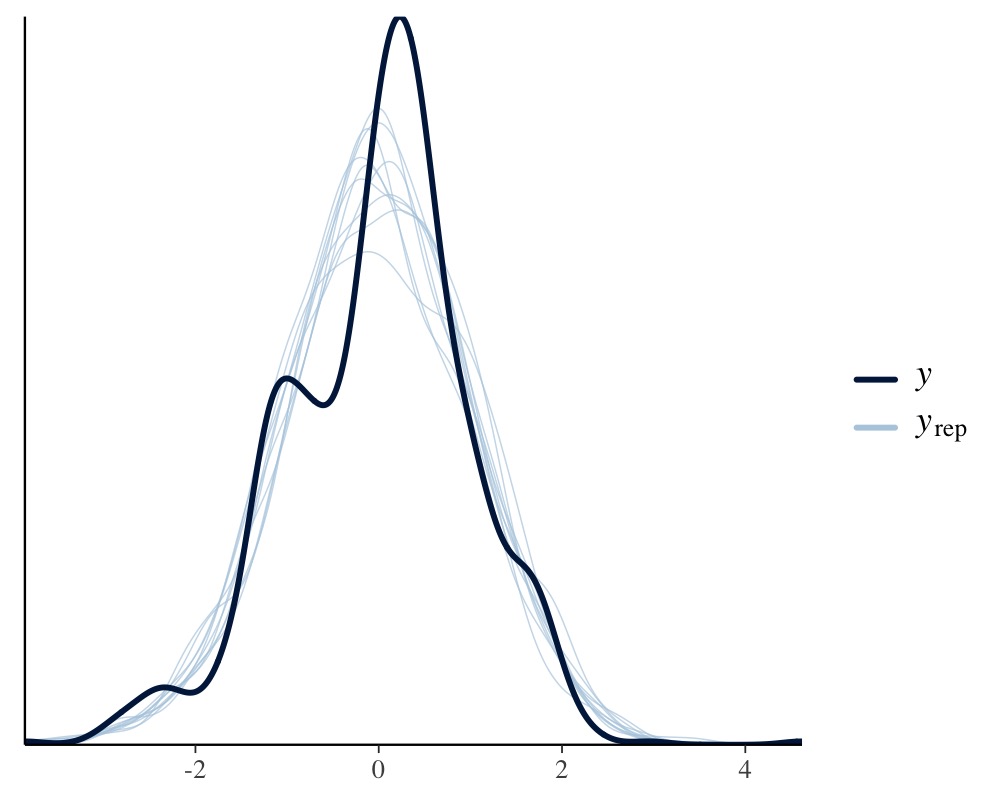
pp_check(fit1, resp = "back")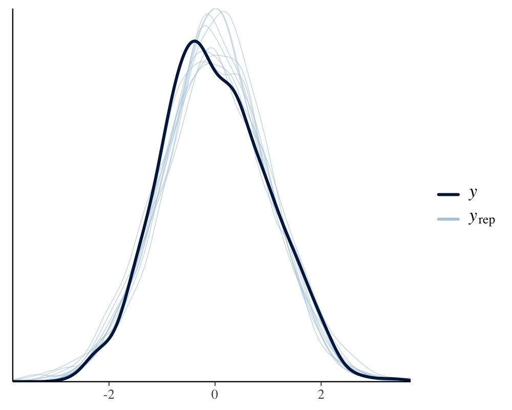
This looks pretty solid, but we notice a slight unmodeled left
skewness in the distribution of tarsus. We will come back
to this later on. Next, we want to investigate how much variation in the
response variables can be explained by our model and we use a Bayesian
generalization of the \(R^2\)
coefficient.
bayes_R2(fit1) Estimate Est.Error Q2.5 Q97.5
R2tarsus 0.4340333 0.02576654 0.3828355 0.4812322
R2back 0.1989010 0.02925046 0.1421987 0.2565427Clearly, there is much variation in both animal characteristics that we can not explain, but apparently we can explain more of the variation in tarsus length than in back color.
More Complex Multivariate Models
Now, suppose we only want to control for sex in
tarsus but not in back and vice versa for
hatchdate. Not that this is particular reasonable for the
present example, but it allows us to illustrate how to specify different
formulas for different response variables. We can no longer use
mvbind syntax and so we have to use a more verbose
approach:
bf_tarsus <- bf(tarsus ~ sex + (1|p|fosternest) + (1|q|dam))
bf_back <- bf(back ~ hatchdate + (1|p|fosternest) + (1|q|dam))
fit2 <- brm(bf_tarsus + bf_back + set_rescor(TRUE),
            data = BTdata, chains = 2, cores = 2)
Note that we have literally added the two model parts via
the + operator, which is in this case equivalent to writing
mvbf(bf_tarsus, bf_back). See
help("brmsformula") and help("mvbrmsformula")
for more details about this syntax. Again, we summarize the model
first.
fit2 <- add_criterion(fit2, "loo")
summary(fit2)
Family: MV(gaussian, gaussian)
Links: mu = identity
mu = identity
Formula: tarsus ~ sex + (1 | p | fosternest) + (1 | q | dam)
back ~ hatchdate + (1 | p | fosternest) + (1 | q | dam)
Data: BTdata (Number of observations: 828)
Draws: 2 chains, each with iter = 2000; warmup = 1000; thin = 1;
total post-warmup draws = 2000
Multilevel Hyperparameters:
~dam (Number of levels: 106)
Estimate Est.Error l-95% CI u-95% CI Rhat Bulk_ESS
sd(tarsus_Intercept) 0.48 0.05 0.39 0.59 1.00 745
sd(back_Intercept) 0.25 0.08 0.09 0.39 1.01 334
cor(tarsus_Intercept,back_Intercept) -0.50 0.22 -0.94 -0.07 1.00 535
Tail_ESS
sd(tarsus_Intercept) 1155
sd(back_Intercept) 573
cor(tarsus_Intercept,back_Intercept) 647
~fosternest (Number of levels: 104)
Estimate Est.Error l-95% CI u-95% CI Rhat Bulk_ESS
sd(tarsus_Intercept) 0.27 0.05 0.16 0.38 1.00 758
sd(back_Intercept) 0.35 0.06 0.22 0.46 1.00 541
cor(tarsus_Intercept,back_Intercept) 0.68 0.20 0.21 0.98 1.00 301
Tail_ESS
sd(tarsus_Intercept) 1310
sd(back_Intercept) 991
cor(tarsus_Intercept,back_Intercept) 530
Regression Coefficients:
Estimate Est.Error l-95% CI u-95% CI Rhat Bulk_ESS Tail_ESS
tarsus_Intercept -0.41 0.07 -0.55 -0.28 1.00 1449 1482
back_Intercept 0.00 0.05 -0.11 0.11 1.00 2260 1172
tarsus_sexMale 0.77 0.06 0.66 0.89 1.00 3576 1579
tarsus_sexUNK 0.22 0.13 -0.03 0.48 1.00 2967 1536
back_hatchdate -0.09 0.05 -0.19 0.02 1.00 2317 1424
Further Distributional Parameters:
Estimate Est.Error l-95% CI u-95% CI Rhat Bulk_ESS Tail_ESS
sigma_tarsus 0.76 0.02 0.72 0.80 1.00 2306 1722
sigma_back 0.90 0.02 0.86 0.95 1.00 1752 1186
Residual Correlations:
Estimate Est.Error l-95% CI u-95% CI Rhat Bulk_ESS Tail_ESS
rescor(tarsus,back) -0.05 0.04 -0.12 0.02 1.00 3167 1632
Draws were sampled using sampling(NUTS). For each parameter, Bulk_ESS
and Tail_ESS are effective sample size measures, and Rhat is the potential
scale reduction factor on split chains (at convergence, Rhat = 1).Let’s find out, how model fit changed due to excluding certain effects from the initial model:
loo(fit1, fit2)Output of model 'fit1':
Computed from 2000 by 828 log-likelihood matrix.
Estimate SE
elpd_loo -2127.5 33.7
p_loo 177.4 7.5
looic 4255.0 67.4
------
MCSE of elpd_loo is NA.
MCSE and ESS estimates assume MCMC draws (r_eff in [0.4, 1.9]).
Pareto k diagnostic values:
Count Pct. Min. ESS
(-Inf, 0.7] (good) 827 99.9% 92
(0.7, 1] (bad) 1 0.1% <NA>
(1, Inf) (very bad) 0 0.0% <NA>
See help('pareto-k-diagnostic') for details.
Output of model 'fit2':
Computed from 2000 by 828 log-likelihood matrix.
Estimate SE
elpd_loo -2124.6 33.6
p_loo 174.3 7.4
looic 4249.2 67.2
------
MCSE of elpd_loo is NA.
MCSE and ESS estimates assume MCMC draws (r_eff in [0.4, 1.7]).
Pareto k diagnostic values:
Count Pct. Min. ESS
(-Inf, 0.7] (good) 825 99.6% 106
(0.7, 1] (bad) 3 0.4% <NA>
(1, Inf) (very bad) 0 0.0% <NA>
See help('pareto-k-diagnostic') for details.
Model comparisons:
model elpd_diff se_diff p_worse diag_diff diag_elpd
fit2 0.0 0.0 NA 3 k_psis > 0.7
fit1 -2.9 1.3 0.99 |elpd_diff| < 4 1 k_psis > 0.7Apparently, there is no noteworthy difference in the model fit.
Accordingly, we do not really need to model sex and
hatchdate for both response variables, but there is also no
harm in including them (so I would probably just include them).
To give you a glimpse of the capabilities of brms’
multivariate syntax, we change our model in various directions at the
same time. Remember the slight left skewness of tarsus,
which we will now model by using the skew_normal family
instead of the gaussian family. Since we do not have a
multivariate normal (or student-t) model, anymore, estimating residual
correlations is no longer possible. We make this explicit using the
set_rescor function. Further, we investigate if the
relationship of back and hatchdate is really
linear as previously assumed by fitting a non-linear spline of
hatchdate. On top of it, we model separate residual
variances of tarsus for male and female chicks.
bf_tarsus <- bf(tarsus ~ sex + (1|p|fosternest) + (1|q|dam)) +
  lf(sigma ~ 0 + sex) + skew_normal()
bf_back <- bf(back ~ s(hatchdate) + (1|p|fosternest) + (1|q|dam)) +
  gaussian()

fit3 <- brm(
  bf_tarsus + bf_back + set_rescor(FALSE),
  data = BTdata, chains = 2, cores = 2,
  control = list(adapt_delta = 0.95)
)
Again, we summarize the model and look at some posterior-predictive checks.
fit3 <- add_criterion(fit3, "loo")
summary(fit3)
Family: MV(skew_normal, gaussian)
Links: mu = identity; sigma = log
mu = identity
Formula: tarsus ~ sex + (1 | p | fosternest) + (1 | q | dam)
sigma ~ 0 + sex
back ~ s(hatchdate) + (1 | p | fosternest) + (1 | q | dam)
Data: BTdata (Number of observations: 828)
Draws: 2 chains, each with iter = 2000; warmup = 1000; thin = 1;
total post-warmup draws = 2000
Smoothing Spline Hyperparameters:
Estimate Est.Error l-95% CI u-95% CI Rhat Bulk_ESS Tail_ESS
sds(back_shatchdate_1) 1.94 1.04 0.29 4.35 1.01 372 310
Multilevel Hyperparameters:
~dam (Number of levels: 106)
Estimate Est.Error l-95% CI u-95% CI Rhat Bulk_ESS
sd(tarsus_Intercept) 0.47 0.05 0.38 0.58 1.00 748
sd(back_Intercept) 0.23 0.07 0.11 0.37 1.00 343
cor(tarsus_Intercept,back_Intercept) -0.54 0.23 -0.95 -0.08 1.00 478
Tail_ESS
sd(tarsus_Intercept) 1304
sd(back_Intercept) 798
cor(tarsus_Intercept,back_Intercept) 569
~fosternest (Number of levels: 104)
Estimate Est.Error l-95% CI u-95% CI Rhat Bulk_ESS
sd(tarsus_Intercept) 0.26 0.05 0.16 0.37 1.00 524
sd(back_Intercept) 0.32 0.06 0.21 0.44 1.00 555
cor(tarsus_Intercept,back_Intercept) 0.64 0.21 0.17 0.97 1.00 267
Tail_ESS
sd(tarsus_Intercept) 918
sd(back_Intercept) 1167
cor(tarsus_Intercept,back_Intercept) 646
Regression Coefficients:
Estimate Est.Error l-95% CI u-95% CI Rhat Bulk_ESS Tail_ESS
tarsus_Intercept -0.41 0.07 -0.54 -0.27 1.00 1116 1436
back_Intercept 0.00 0.05 -0.09 0.10 1.00 1563 1618
tarsus_sexMale 0.77 0.06 0.65 0.88 1.01 3207 1221
tarsus_sexUNK 0.22 0.12 -0.02 0.45 1.00 3000 1438
sigma_tarsus_sexFem -0.30 0.04 -0.38 -0.22 1.00 2456 1384
sigma_tarsus_sexMale -0.25 0.04 -0.32 -0.17 1.00 2733 1579
sigma_tarsus_sexUNK -0.40 0.13 -0.64 -0.14 1.00 2005 1689
back_shatchdate_1 -0.32 3.08 -5.79 6.54 1.00 1293 1356
Further Distributional Parameters:
Estimate Est.Error l-95% CI u-95% CI Rhat Bulk_ESS Tail_ESS
sigma_back 0.90 0.02 0.85 0.95 1.00 2361 1363
alpha_tarsus -1.20 0.46 -1.89 0.22 1.00 939 345
Draws were sampled using sampling(NUTS). For each parameter, Bulk_ESS
and Tail_ESS are effective sample size measures, and Rhat is the potential
scale reduction factor on split chains (at convergence, Rhat = 1).We see that the (log) residual standard deviation of
tarsus is somewhat larger for chicks whose sex could not be
identified as compared to male or female chicks. Further, we see from
the negative alpha (skewness) parameter of
tarsus that the residuals are indeed slightly left-skewed.
Lastly, running
conditional_effects(fit3, "hatchdate", resp = "back")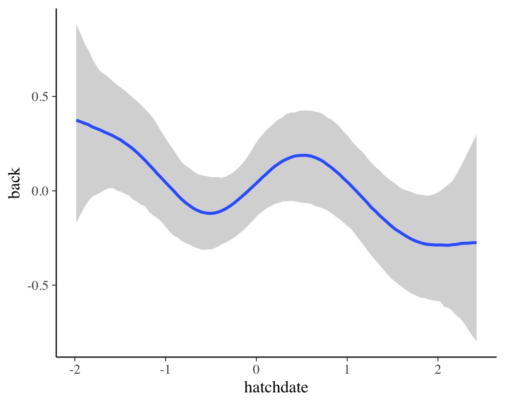
reveals a non-linear relationship of hatchdate on the
back color, which seems to change in waves over the course
of the hatch dates.
There are many more modeling options for multivariate models, which
are not discussed in this vignette. Examples include autocorrelation
structures, Gaussian processes, or explicit non-linear predictors (e.g.,
see help("brmsformula") or
vignette("brms_multilevel")). In fact, nearly all the
flexibility of univariate models is retained in multivariate models.